Today we talk about the very frequent problems that occur in machine learning: overfitting and regularization. Let's briefly understand the commonly used L0, L1, L2 and kernel norm regularization. Finally, let's talk about the selection of regularization parameters. Because the space here is relatively large, in order not to scare everyone, I will divide these five parts into two blog posts. Knowledge is limited. The following are my simple ideas. If there are errors in understanding, I hope everyone can correct them. Thank you.

       The problem of supervised machine learning is nothing more than "minimizeyour error while regularizing your parameters", which is to minimize errors while regularizing parameters. Minimizing errors is to allow our model to fit our training data, and regularization parameters are to prevent our model from overfitting our training data. What a minimalistic philosophy! Because too many parameters will cause our model to increase in complexity and easy to overfit, that is, our training error will be small. But small training error is not our ultimate goal. Our goal is to hope that the test error of the model is small, that is, it can accurately predict new samples. Therefore, we need to ensure that the model is "simple" to minimize training errors, so that the parameters obtained have good generalization performance (that is, the test error is also small), and the model "simple" is implemented by a rule function. In addition, the use of rule terms can also constrain the characteristics of our model. In this way, people's prior knowledge of this model can be incorporated into the learning of the model, and the learned model can be forced to have the characteristics that people want, such as sparse, low rank, smooth, and so on. You know, sometimes human transcendent is very important. The previous experience will make you take a lot less detours, which is why we usually learn to find a big cow belt. A few clicks can clear the dark clouds before us, and return us a clear sky. The same is true for machine learning. If we are dialed a little by us, it will definitely learn the corresponding task faster. It is only because there is no such direct method for human-machine communication. At present, this medium can only be played by rules.

       There are also several perspectives on regularization. Regularization conforms to Occam's razor principle. This name is so domineering, razor! However, the idea is very approachable: Of all the models that can be selected, we should choose a model that can explain the known data well and is very simple. From the perspective of Bayesian estimation, the regularization term corresponds to the prior probability of the model. There is another saying in the folk that regularization is the realization of the structural risk minimization strategy, which is to add a regularizer or penalty term to the empirical risk.

       In general, supervised learning can be seen as minimizing the following objective function:

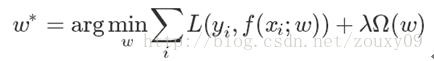
       Wherein the first L (Y i , F (X i ; W)) (X measure our model (classification or regression) on the i-th sample predicted value F i ; W) and a true labels Y i before error. Because our model is to fit our training samples, we require this item to be the smallest, that is, our model needs to fit our training data as much as possible. But as said above, we not only want to ensure the minimum training error, we also want our model test error to be small, so we need to add the second term, which is the regularization function Ω (w) for the parameter w to constrain our The model is as simple as possible.

       OK, here, if you have been fighting in machine learning for many years, you will find that, oh, most of the models with parameters in machine learning are not only similar to this, but also godlike. Yes, in fact, most of them are nothing more than transforming these two items. For the first Loss function, if it is Square loss, it is least squares; if it is Hinge Loss, it is the famous SVM; if it is exp-Loss, it is a powerful boosting; if it is log-los That's Logistic Regression; wait a minute. Different loss functions have different fitting characteristics, and this has to be analyzed specifically for specific problems. But here, we don't study the problem of loss function first, we turn our attention to the "regular term Ω (w)".

       There are also many options for the regularization function Ω (w), which is generally a monotonically increasing function of model complexity. The more complex the model, the larger the regularization value. For example, the regularization term can be the norm of a model parameter vector. However, different choices have different constraints on the parameter w, and the results obtained are different, but we often gather in the paper: zero norm, first norm, second norm, trace norm, Frobenius norm, and kernel Norms and so on. With so many norms, what do they mean? What ability? When will it be available? When should I use it? No hurry, let's pick a few common martyrdom.

First, L0 norm and L1 norm

       The L0 norm refers to the number of non-zero elements in the vector. If we use the L0 norm to regularize a parameter matrix W, we hope that most elements of W are 0. This is too intuitive, too explicit, in other words, let the parameter W be sparse. OK, seeing the word "sparse", everyone should wake up from the current "compressive perception" and "sparse coding". The original "sparseness" of the mountains and mountains is used to achieve this. But you start to doubt again, is that so? In the papers world you see, isn't sparseness achieved through the L1 norm? Is my mind everywhere? || W || 1 shadow! It is almost impossible to look up. That's right, that's why the title of this section put L0 and L1 together, because they have some kind of unusual relationship. Let's see what the L1 norm is again? Why can it achieve sparseness? Why does everyone use the L1 norm to achieve sparseness instead of the L0 norm?

       The L1 norm refers to the sum of the absolute values ​​of the elements in a vector. It is also known as a "Lasso regularization operator." Now let's analyze this one hundred million question: Why does the L1 norm make the weights sparse? Someone might answer this "It is the optimal convex approximation of the L0 norm". In fact, there is a more beautiful answer: Any regularization operator, if he W i = 0 where non-differentiable and can be broken down into a "sum" form, then the rules of the operator can be achieved Sparse. This is to say, the L1 norm of W is an absolute value, | w | is not differentiable at w = 0, but this is still not intuitive enough. This is because we need to compare and analyze with the L2 norm. So for an intuitive understanding of the L1 norm, check out the second section later.

       By the way, there is another question above: Since L0 can be sparse, why not use L0 and use L1 instead? My personal understanding is that the L0 norm is difficult to optimize and solve (NP difficult problem), and the second is that the L1 norm is the optimal convex approximation of the L0 norm, and it is easier to optimize than the L0 norm. That's why everyone turned their eyes and thousands of pets on the L1 norm.

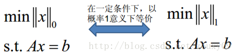
       OK, to summarize in one sentence: L1 norm and L0 norm can achieve sparseness, L1 is widely used because it has better optimization solution characteristics than L0.

       Ok, so here, we probably know that L1 can be sparse, but we will think, why should it be sparse? What's the benefit of making our parameters sparse? Here are two points:

1) Feature Selection:

       One of the key reasons why everyone is rushing to sparse regularization is that it enables automatic selection of features. In general, most of the elements of x i (that is, features) are not related to the final output y i or provide no information. When minimizing the objective function, consider these additional features of x i . Smaller training error, but when predicting new samples, this useless information will be considered instead, which will interfere with the prediction of the correct y i . The introduction of the sparse regularization operator is to fulfill the glorious mission of automatic feature selection. It will learn to remove these features without information, that is, reset the weights corresponding to these features to 0.

2) Interpretability:

       Another reason for sparseness is that models are easier to explain. For example, the probability of suffering from a certain disease is y, and then the data x we ​​collect is 1000 dimensions, that is, we need to find out how these 1000 factors affect the probability of suffering from this disease. Suppose we are a regression model: y = w 1 * x 1 + w 2 * x 2 + ... + w 1000 * x 1000 + b (Of course, in order to limit y to the range of [0,1], we generally have to Add a Logistic function). Through learning, if the last learned w * has only a few non-zero elements, such as only 5 non-zero w i , then we have reason to believe that the information provided by these corresponding features in the disease analysis is huge Decision-making. In other words, whether or not the disease is affected is only related to these 5 factors, and the doctor is better to analyze. But if 1000 w i are not 0, the doctor will not feel love when faced with these 1000 factors.

Second, L2 norm

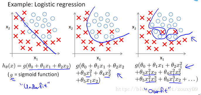
       In addition to the L1 norm, a more favored regularization norm is the L2 norm: || W || 2 . It is not inferior to the L1 norm. It has two good names. In regression, some people call the regression with it "Ridge Regression", and some people call it "weight decay." This is used a lot, because its powerful effect is to improve a very important problem in machine learning: overfitting. As for what overfitting is, it is explained above that the error during model training is small, but the error during testing is very large, that is, our model is complex enough to fit all our training samples, but in When actually predicting a new sample, it was a mess. Popularly speaking, the ability to take exams is very strong, and the actual application ability is poor. Good at memorizing knowledge, but not flexible use of knowledge. For example, as shown below (from Ng's course):

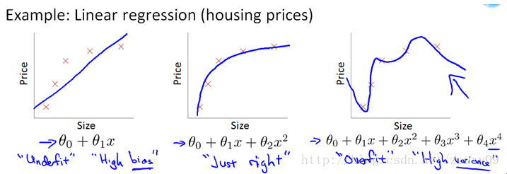
       The upper graph is linear regression, and the lower graph is logistic regression, which can also be said to be the case of classification. From left to right, there are three cases of underfitting (also known as High-bias), suitable fitting and overfitting (also known as High variance). It can be seen that if the model is complex (it can fit arbitrary complex functions), it can let our model fit all data points, that is, there is basically no error. For regression, our function curve passed all the data points, as shown in the right of the figure above. For classification, our function curve must classify all the data points correctly, as shown in the right of the figure below. Both cases are clearly overfitting.

       OK, now we have a very critical question, why can the L2 norm prevent overfitting? Before answering this question, we must first look at what the L2 norm is.

       The L2 norm is the sum of the squares of the elements of the vector and then the square root. We minimize the rule term of the L2 norm || W || 2 to make each element of W small and close to 0, but unlike the L1 norm, it does not make it equal to 0, but close to At 0, there is a big difference here. The smaller the parameter, the simpler the model, and the simpler the model, the less likely it is to overfit. Why is the smaller parameter the simpler the model? I also do n’t understand. My understanding is that limiting the parameters is very small, actually limiting the impact of some components of the polynomial to a small extent (see the fitted graph of the linear regression model above), which is equivalent to reducing the parameters Number. In fact, I don't know much, I hope everyone can give pointers.

       Here is a sentence to sum up: through the L2 norm, we can achieve the limit on the model space, thereby avoiding overfitting to a certain extent.

       What are the benefits of the L2 norm? There are two points here:

1) Learning theory perspective:

       From the perspective of learning theory, the L2 norm can prevent overfitting and improve the generalization ability of the model.

2) Optimized calculation angle:

       From the perspective of optimization or numerical calculation, the L2 norm is helpful to deal with the problem that matrix inversion is difficult when the condition number is bad. Hey, wait, what is this condition number? I google it first.

       Here we pretend to be elegant to talk about optimization problems. There are two major problems in optimization, one is the local minimum, and the other is the ill-condition problem. The former 俺 will not talk about it, everyone understands that we are looking for a global minimum. If there are too many local minimums, then our optimization algorithm can easily fall into local minimums and cannot extricate themselves. This is obviously not an audience willing To the plot. Then let's talk about ill-condition. ill-condition corresponds to well-condition. What do they represent? Suppose we have a system of equations AX = b and we need to solve X. If A or b changes slightly, the solution of X will change greatly, then the system of equations is ill-condition, otherwise it is well-condition. Let's take an example:

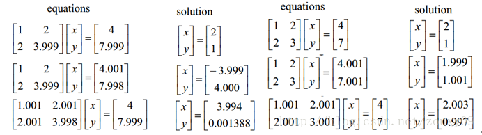
       Let's look at the one on the left first. The first line assumes that we have AX = b. In the second line, we change b slightly, and the obtained x is very different from before. See it. In the third line, we change the coefficient matrix A slightly, and we can see that the results also change a lot. In other words, the solution of this system is too sensitive to the coefficient matrix A or b. Also, because our coefficient matrices A and b are generally estimated from experimental data, there is an error. If our system can tolerate this error, it is good, but the system is too sensitive to this error. So that the error of our solution is greater, then this solution is too unreliable. So this system of equations is ill-conditioned, abnormal, unstable, problematic, haha. This is clear. The one on the right is called the well-condition system.

       Let's talk about it again. For an ill-condition system, my input changes slightly, and the output changes a lot. This is not good, which indicates that our system is not practical. If you think about it, for example, for a regression problem y = f (x), we use the training sample x to train the model f so that y outputs the value we expect, such as 0. So if we encounter a sample x ', this sample is very different from the training sample x. In the face of him, the system should output a value similar to the above y, such as 0.00001, but it finally outputs me a 0.9999. Obviously wrong. It's like, a person with whom you are familiar has acne on your face, and you don't know him, then your brain is too bad, haha. So if a system is ill-conditioned, we will doubt its results. So how much do you have to believe it? We have to find a standard to measure it, because some systems are not so serious, and the results can still be trusted, not across the board. Finally back, the above condition number is used to measure the credibility of the ill-condition system. The condition number measures how much the output changes when the input changes slightly. That is, the sensitivity of the system to small changes. A small condition number value is well-conditioned, and a large value is ill-conditioned.

       If the square matrix A is non-singular, then the conditionnumber of A is defined as:

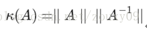
       That is, the norm of matrix A times its inverse norm. So the specific value depends on what norm you choose. If the square matrix A is singular, then the condition number of A is positive infinity. In fact, each reversible square has a condition number. But to calculate it, we need to know the norm (norm) and Machine Epsilon (machine precision) of this square matrix. Why norm? Norm is equivalent to measuring the size of a matrix. We know that a matrix has no size. When the above is not to measure a matrix A or a vector b, does our solution x change? So there must be something to measure the size of matrices and vectors, right? By the way, he is the norm, which means the size of the matrix or the length of the vector. OK, after a relatively simple proof, for AX = b, we can get the following conclusions:

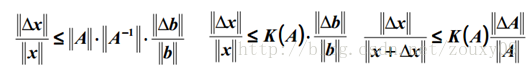
       That is, the relative change of our solution x and the relative change of A or b have the same relationship as above, where the value of k (A) is equivalent to the magnification, see? Equivalent to the bound of x change.

       Summarize the condition number in one sentence: conditionnumber is a measure of the stability or sensitivity of a matrix (or the linear system it describes). If a matrix's condition number is near 1, it is well-conditioned. If it is much larger than 1, then it is ill-conditioned. If a system is ill-conditioned, its output should not be trusted too much.

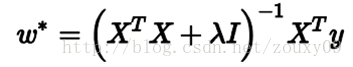
       Okay, so much has been said about such a thing. By the way, why did we talk about this? Going back to the first sentence: From the perspective of optimization or numerical calculation, the L2 norm is helpful to deal with the problem that matrix inversion is difficult when the condition number is not good. Because if the objective function is quadratic, for linear regression, there is actually an analytical solution. Finding the derivative and making the derivative equal to zero gives the optimal solution as:

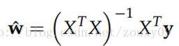
       However, if the number of our samples X is smaller than the dimensions of each sample, the matrix X T X will not be full rank, that is, X T X will become irreversible, so w * cannot be directly Calculated. Or rather, there will be infinitely many solutions (because the number of our equations is less than the number of unknowns). In other words, our data is not enough to determine a solution. If we randomly choose one from all feasible solutions, it may not be a really good solution. In short, we are overfitting.

       But if you add the L2 rule, it becomes the following situation, and you can directly invert:

       Here, the description of the professional point is: To obtain this solution, we usually do not directly find the inverse of the matrix, but calculate it by solving linear equations (such as the Gaussian elimination method). Considering the case where there is no rule term, that is, λ = 0, if the condition number of the matrix X T X is large, the solution of linear equations will be numerically unstable, and the introduction of this rule term can improve the condition number.

       In addition, if you use an iterative optimization algorithm, a too large condition number will still cause problems: it will slow down the convergence speed of the iteration, and from the perspective of optimization, the rule term actually turns the objective function into λ-strongly convex ( λ is strongly convex). Oops, here is another λ strong convex. What is λ strong convex?

       When f satisfies:

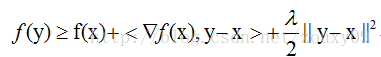
       , We call f a λ-stronglyconvex function, where the parameter λ> 0. When λ = 0, it returns to the definition of ordinary convex function.

       Before visually explaining strong convexity, let's see what ordinary convexity looks like. Suppose we let f make a first-order Taylor approximation at x (do you forget the first-order Taylor expansion? F (x) = f (a) + f '(a) (xa) + o (|| xa ||)). ):

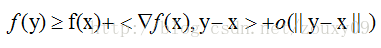
       Intuitively speaking, the convex property refers to the tangent of the function curve at that point, that is, above the linear approximation, and strongly convex further requires that it be above a quadratic function at that point, which means that the function is not too "flat" Rather, it can guarantee a certain "bending upward" trend. Professionally speaking, it is that convex can guarantee that the function is above its first-order Taylor function at any point, and strongly convex can ensure that the function has a very beautiful quadratic lower bound at any point. Of course this is a strong assumption, but it is also a very important assumption. It may not be easy to understand, let's draw a picture to understand it visually.

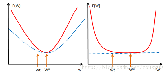
       As soon as you see the picture above, you understand everything. Don't need me to slap it. Let's talk about it. Where we take our optimal solution w *. If our function f (w) is shown on the left, that is, the red function will be above the quadratic function of the blue dotted line, so even if w t and w * are closer, f (w The value of t ) and f (w *) are quite different, that is, there will be a large gradient value near our optimal solution w *, so that we can have fewer iterations. Within w *. But for the right picture, the red function f (w) is only constrained above a linear blue dotted line. Assuming it is the unfortunate situation (very flat) like the right picture, then w t is still our best advantage w * At a long distance, our approximate gradient (f (w t ) -f (w *)) / (w t -w *) is already very small, and the approximate gradient ∂f / ∂w at w t is It is smaller, so through gradient descent w t + 1 = w t -α * (∂f / ∂w), we get the result that w changes very slowly, like a snail, very slowly to our best advantage w * Crawling, it is still far from our best advantage in a limited iteration time.

       So just relying on the nature of convex does not guarantee that the point w obtained under the conditions of gradient descent and a limited number of iterations will be a better approximation point of the global minimum point w *. Stopping near the optimum is also a way to regularize or improve generalization performance). As analyzed above, if f (w) is very flat around the global minimum point w *, we may find a far point. But if we have "strong convexity", we can control the situation and we can get a better approximate solution. As for how good it is, there is a bound in it, the quality of this bound also depends on the size of the constant α in the strongly convex property. Seeing this, I don't know if everyone is smart. What if you want to get strongly convex? The simplest is to add an item (α / 2) * || w || 2 to it .

       Uh, it took so much to talk about a strongly convex. In fact, in gradient descent, the upper bound of the convergence rate of the objective function is actually related to the condition number of the matrix X T X. The smaller the condition number of X T X, the smaller the upper bound, that is, the faster the convergence rate .

This one optimization says so much. Let's summarize it in a sentence: the L2 norm not only prevents overfitting, but also makes our optimization solution stable and fast.

       Well, here is to fulfill the promises above, and let's talk about the difference between L1 and L2 intuitively. Why is there such a big difference when one minimizes the absolute value and one minimizes the square? I see two geometrically intuitive resolutions:

1) Falling speed:

       We know that both L1 and L2 are regular methods. We put the weight parameters into the cost function in the way of L1 or L2. The model then tries to minimize these weight parameters. And this minimization is like a downhill process. The difference between L1 and L2 lies in this "slope", as shown in the figure below: L1 is descended according to the "slope" of the absolute value function, while L2 is descended according to the "quadratic function" "Slope". So in fact, near 0, the falling speed of L1 is faster than the falling speed of L2. So it will drop to 0 very quickly. However, I think the explanation here is not very relevant. Of course, I don't know if it is a problem I understand.

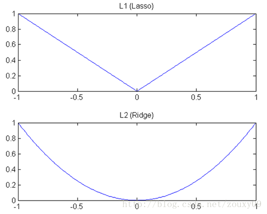
       L1 is called Lasso on the rivers and lakes, and L2 is called Ridge. However, these two names are quite confusing. Looking at the picture above, Lasso's picture looks like ridge, and ridge's picture looks like lasso.

2) Limitations of model space:

       In fact, for L1 and L2 regularized cost functions, we can write the following:

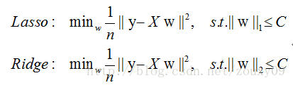
       That is, we limit the model space to a L1-ball of w. In order to facilitate visualization, we consider a two-dimensional situation. Contour lines of the objective function can be drawn on the (w1, w2) plane, and the constraint condition is a norm ball with a radius C on the plane. The optimal solution is where the contour line intersects the norm ball for the first time:

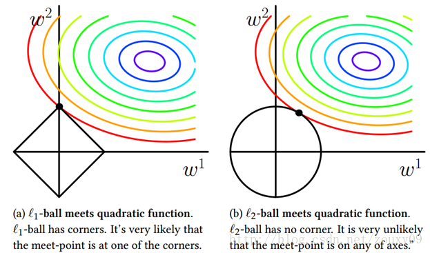
       It can be seen that the difference between L1-ball and L2-ball is that L1 has an "angle" where it intersects with each coordinate axis, and the geodesic of the objective function will be most of the time unless the position is very well Intersect at the corner. Note that sparsity occurs at the corner position, for example, the intersection point in the figure has w1 = 0, and when it is higher dimensional (Imagine what a three-dimensional L1-ball looks like?) In addition to the corner point, Contours with many edges also have a high probability of becoming the first place to intersect, and will produce sparsity.

       In contrast, L2-ball has no such property, because there is no corner, so the probability of the first intersection place appearing in a sparse location becomes very small. This intuitively explains why L1-regularization can produce sparseness, but L2-regularization cannot.

       Therefore, a sentence summary is: L1 tends to produce a small number of features, while other features are 0, and L2 will choose more features, these features will be close to 0. Lasso is very useful in feature selection, and Ridge is just a regularization.

       OK, here we go. In the next blog post, we talk about the issue of kernel norms and regularization parameter selection. For the full reference material, please also see the next blog post, which is not repeated here. Thank you.

আজ আমরা খুব ঘন ঘন সমস্যাগুলি নিয়ে কথা বলি যা মেশিন লার্নিংয়ে ঘটে: অতিরিক্ত মানানসই ও নিয়মিতকরণ। আসুন সংক্ষেপে সাধারণভাবে ব্যবহৃত L0, L1, L2 এবং কার্নেল আদর্শ নিয়মিতকরণ বুঝতে পারি। পরিশেষে, আসুন নিয়মিতকরণ পরামিতিগুলির নির্বাচন সম্পর্কে কথা বলি। কারণ এখানে স্থান তুলনামূলকভাবে বড়, সবাইকে ভয় না দেওয়ার জন্য, এই পাঁচটি অংশটি দুটি ব্লগ পোস্টে ভাগ করব। জ্ঞান সীমাবদ্ধ The নীচেরগুলি আমার সাধারণ ধারণা। ধন্যবাদ

       তত্ত্বাবধানে থাকা মেশিন লার্নিংয়ের সমস্যাটি "আপনার পরামিতিগুলি নিয়মিত করার সময় আপনার ত্রুটি হ্রাস করা" ছাড়া আর কিছুই নয়, যা পরামিতিগুলিকে নিয়মিত করার সময় ত্রুটিগুলি হ্রাস করতে হয়। ত্রুটিগুলি হ্রাস করা হ'ল আমাদের মডেলটিকে আমাদের প্রশিক্ষণের ডেটা ফিট করতে দেয় এবং নিয়মিতকরণের পরামিতিগুলি হ'ল আমাদের মডেলটিকে আমাদের প্রশিক্ষণের ডেটার চেয়ে বেশি মানিয়ে আটকানো। কি সংক্ষিপ্ত দর্শন! কারণ অনেকগুলি পরামিতিগুলি আমাদের মডেলকে জটিলতা বৃদ্ধি করতে এবং অতিরিক্ত পরিমাণে সহজ করতে সক্ষম করবে, তা হল, আমাদের প্রশিক্ষণের ত্রুটিটি ছোট হবে small তবে ছোট প্রশিক্ষণের ত্রুটিটি আমাদের চূড়ান্ত লক্ষ্য নয় Our আমাদের লক্ষ্যটি আশা করা যায় যে মডেলের পরীক্ষার ত্রুটিটি ছোট, অর্থাৎ এটি সঠিকভাবে নতুন নমুনাগুলি পূর্বাভাস দিতে পারে। অতএব, আমাদের প্রশিক্ষণ ত্রুটিগুলি হ্রাস করতে মডেলটি "সাধারণ" তা নিশ্চিত করতে হবে, যাতে প্রাপ্ত প্যারামিটারগুলিতে ভাল সাধারণীকরণের পারফরম্যান্স থাকতে পারে (যা, পরীক্ষার ত্রুটিটিও ছোট), এবং "সাধারণ" মডেলটি একটি নিয়ম ফাংশন দ্বারা প্রয়োগ করা হয়। তদতিরিক্ত, বিধি শর্তাদি ব্যবহার আমাদের মডেলের বৈশিষ্ট্যগুলিকেও সীমাবদ্ধ করতে পারে। এইভাবে, এই মডেল সম্পর্কে লোকদের পূর্বের জ্ঞানটি মডেলটির শিক্ষার সাথে সংযুক্ত করা যেতে পারে এবং শিখে নেওয়া মডেলটিকে লোকেরা যে বৈশিষ্ট্যগুলি চায়, যেমন স্পারস, নিম্ন স্তরের, মসৃণ ইত্যাদি থাকতে বাধ্য করা যেতে পারে। আপনি জানেন, কখনও কখনও মানুষের অতীত খুব গুরুত্বপূর্ণ। পূর্ববর্তী অভিজ্ঞতা আপনাকে অনেক কম ঘুরে বেড়াতে বাধ্য করবে, এ কারণেই আমরা সাধারণত একটি বড় গরুর বেল্ট খুঁজতে শিখি। কয়েকটি ক্লিক আমাদের আগে অন্ধকার মেঘ পরিষ্কার করতে পারে এবং আমাদের পরিষ্কার আকাশে ফিরিয়ে দিতে পারে। মেশিন লার্নিংয়ের ক্ষেত্রেও এটি একই রকম If আমরা যদি আমাদের দ্বারা কিছুটা ডায়াল করে থাকি তবে এটি অবশ্যই সংশ্লিষ্ট কাজটি দ্রুত শিখবে। এটি কেবলমাত্র কারণ হ'ল মানব-মেশিন যোগাযোগের জন্য এ জাতীয় কোনও সরাসরি পদ্ধতি নেই present বর্তমানে, এই মাধ্যমটি কেবল বিধি দ্বারা চালানো যেতে পারে।

       নিয়মিতকরণের বিষয়েও বেশ কয়েকটি দৃষ্টিভঙ্গি রয়েছে। নিয়মিতকরণ ওকামের ক্ষুরের নীতির সাথে সামঞ্জস্য করে। এই নামটি এতটাই দাপট, রেজার! যাইহোক, ধারণাটি খুব সহজলভ্য: যে সমস্ত মডেল নির্বাচন করা যেতে পারে তার মধ্যে আমাদের এমন একটি মডেল নির্বাচন করা উচিত যা পরিচিত তথ্যগুলি ভালভাবে ব্যাখ্যা করতে পারে এবং খুব সহজ। বায়েশিয়ান অনুমানের দৃষ্টিকোণ থেকে, নিয়ামককরণ শব্দটি মডেলের পূর্ব সম্ভাবনার সাথে মিলে যায়। লোকের মধ্যে আরও একটি বক্তব্য রয়েছে যে নিয়মিতকরণ হ'ল কাঠামোগত ঝুঁকি হ্রাস কৌশলের বাস্তবায়ন, যা বোধগম্য ঝুঁকিতে একটি নিয়ামক বা পেনাল্টি শব্দ যুক্ত করা হয়।

       সাধারণভাবে, তত্ত্বাবধানে পড়াশুনাটি নিম্নলিখিত উদ্দেশ্য কার্যকে হ্রাস হিসাবে দেখা যায়:

       তথায় প্রথম এল (ওয়াই আমি , f (x আমি ; ওয়াট)) (এক্স পরিমাপ আমাদের মডেল (শ্রেণীবিন্যাস বা রিগ্রেশন) আমি তম নমুনা পূর্বাভাস মান এফ উপর আমি ; ডব্লিউ) এবং একটি সত্য লেবেল ওয়াই আমি আগে ত্রুটি। যেহেতু আমাদের মডেলটি আমাদের প্রশিক্ষণের নমুনাগুলির সাথে ফিট করে, তাই আমাদের এই আইটেমটি সবচেয়ে ছোট হওয়া দরকার, এটি হল আমাদের মডেলটিকে আমাদের প্রশিক্ষণের ডেটা যথাসম্ভব ফিট করতে হবে। তবে উপরে যেমন বলা হয়েছে, আমরা কেবল ন্যূনতম প্রশিক্ষণের ত্রুটিটিই নিশ্চিত করতে চাই না, আমরা আমাদের মডেল পরীক্ষার ত্রুটিটিও ছোট হতে চাই, তাই আমাদের দ্বিতীয় পদটি যুক্ত করা দরকার, যা আমাদের প্যারামিটারের নিয়মিতকরণ ফাংশন w (ডাব্লু) আমাদের সীমাবদ্ধ করতে হবে মডেল যতটা সম্ভব সহজ।

       ঠিক আছে, এখানে, আপনি যদি বেশ কয়েক বছর ধরে মেশিন লার্নিংয়ে লড়াই করে চলেছেন তবে আপনি দেখতে পাবেন যে ওহ, মেশিন লার্নিংয়ের পরামিতিগুলির বেশিরভাগ মডেলগুলি কেবল এটির মতোই নয়, godশ্বরের মতও। হ্যাঁ, বাস্তবে, তাদের বেশিরভাগই এই দুটি আইটেমকে রূপান্তর করা ছাড়া আর কিছুই নয়। প্রথম ক্ষতির ক্রিয়াকলাপের জন্য, যদি এটি স্কোয়ার ক্ষতি হয় তবে এটি সর্বনিম্ন স্কোয়ার হয়; এটি হিন্জ লস হলে এটি বিখ্যাত এসভিএম; এটি এক্সপ-লস হলে এটি একটি শক্তিশালী উত্সাহদান; যদি এটি লগ-লোকস হয় এটি লজিস্টিক রিগ্রেশন; এক মিনিট অপেক্ষা করুন। বিভিন্ন ক্ষতির বিভিন্ন ফাংশনগুলির বিভিন্ন ফিটিং বৈশিষ্ট্য রয়েছে এবং এটি নির্দিষ্ট সমস্যার জন্য বিশেষত বিশ্লেষণ করতে হবে। তবে এখানে, আমরা ক্ষতির কার্যকারিতাটির সমস্যাটি প্রথমে অধ্যয়ন করি না, আমরা আমাদের "নিয়মিত শব্দ Ω (ডাব্লু)" এর দিকে মনোনিবেশ করি।

       নিয়মিতকরণের জন্য অনেকগুলি বিকল্প রয়েছে w (ডাব্লু), যা সাধারণত মডেল জটিলতার একঘেয়েমি ক্রমবর্ধমান ফাংশন the মডেলটি যত জটিল, নিয়মিতকরণের মান তত বেশি। উদাহরণস্বরূপ, নিয়মিতকরণ শব্দটি কোনও মডেল প্যারামিটার ভেক্টরের আদর্শ হতে পারে। যাইহোক, বিভিন্ন পছন্দগুলির ডাব্লু প্যারামিটারে বিভিন্ন বাধা রয়েছে এবং প্রাপ্ত ফলাফলগুলি পৃথক হয় তবে আমরা প্রায়শই কাগজে জড়ো করি: শূন্য আদর্শ, প্রথম আদর্শ, দ্বিতীয় আদর্শ, ট্রেস নর্ম, ফ্রোবেনিয়াস নর্ম এবং কার্নেল নিয়ম এবং অন্যান্য। অনেক নিয়ম সহ, তাদের অর্থ কী? কি ক্ষমতা? কখন পাওয়া যাবে? আমি কখন এটি ব্যবহার করব? তাড়াহুড়া করবেন না, আসুন কয়েকটি সাধারণ শাহাদাত বাছাই করা যাক।

প্রথমত, L0 আদর্শ এবং L1 আদর্শ

       L0 নিয়মটি ভেক্টরটিতে শূন্য নয় এমন উপাদানগুলির সংখ্যা বোঝায়। যদি আমরা প্যারামিটার ম্যাট্রিক্স ডাব্লু নিয়মিত করতে L0 আদর্শ ব্যবহার করি তবে আমরা আশা করি যে ডাব্লু এর বেশিরভাগ উপাদান 0 হয়। এটি অত্যন্ত স্বজ্ঞাত, খুব স্পষ্ট, অন্য কথায়, ডাব্লু প্যারামিটারটি কম। ঠিক আছে, "স্পার্স" শব্দটি দেখে প্রত্যেকের বর্তমান "সংবেদনশীল উপলব্ধি" এবং "স্পার্স কোডিং" থেকে জেগে ওঠা উচিত the পর্বতমালার পর্বতগুলির মূল "বিরলতা" এটি অর্জন করতে ব্যবহৃত হয়। কিন্তু আপনি আবার সন্দেহ করতে শুরু করেন, তা কি তাই? কাগজপত্রের জগতে আপনি দেখতে পাচ্ছেন, L1 আদর্শের মাধ্যমে স্বল্পতা অর্জন করা যায় না? আমার মন কি সর্বত্র? || ডাব্লু || 1 ছায়া! সন্ধান করা প্রায় অসম্ভব। ঠিক আছে, এই কারণেই এই বিভাগের শিরোনাম L0 এবং L1 কে একসাথে রেখেছিল কারণ তাদের একরকম অস্বাভাবিক সম্পর্ক রয়েছে। আসুন দেখে নেওয়া যাক আবার এল 1 আদর্শ কী? কেন এটি স্বল্পতা অর্জন করতে পারে? সবাই কেন L0 আদর্শের পরিবর্তে অল্প পরিমাণে অর্জন করতে L1 আদর্শ ব্যবহার করে?

       এল 1 আদর্শটি কোনও ভেক্টরের উপাদানগুলির নিখুঁত মানগুলির যোগফলকে বোঝায় It এটি "লাসো নিয়মিতকরণ অপারেটর" নামেও পরিচিত। এবার এই একশ মিলিয়ন প্রশ্নের বিশ্লেষণ করা যাক: এল 1 আদর্শ কেন ওজনকে বিচ্ছিন্ন করে? কেউ এর উত্তর দিতে পারে "এটি L0 আদর্শের সর্বোত্তম উত্তল অনুমান"। আসলে, সেখানে একটি আরো সুন্দর উত্তর: যেকোনো নিয়মিতকরণ অপারেটর, সে যদি ওয়াট আমি = 0 যেখানে অ differentiable এবং একটি "সমষ্টি" ফর্ম বিভক্ত করা যেতে পারে, তারপর অপারেটর নিয়ম অর্জন করা যেতে পারে বিক্ষিপ্ত। এটি বলার অপেক্ষা রাখে না, ডাব্লু এর এল 1 আদর্শ একটি পরম মান, | ডাব্লু | ডাব্লু = 0 এ পার্থক্যযোগ্য নয়, তবে এটি এখনও যথেষ্ট স্বজ্ঞাত নয়। এটি কারণ আমাদের এল 2 আদর্শের সাথে তুলনা এবং বিশ্লেষণ করা দরকার। সুতরাং এল 1 আদর্শ সম্পর্কে স্বজ্ঞাত জ্ঞানের জন্য পরে দ্বিতীয় বিভাগটি দেখুন check

       যাইহোক, উপরে আরও একটি প্রশ্ন রয়েছে: যেহেতু L0 বিচ্ছুরিত হতে পারে, তবে L0 ব্যবহার করবেন না এবং পরিবর্তে L1 ব্যবহার করবেন না কেন? আমার ব্যক্তিগত বোধগম্যতা হল যে L0 আদর্শটি অনুকূল করা এবং সমাধান করা (এনপি কঠিন সমস্যা), এবং দ্বিতীয়টি হল L1 আদর্শটি L0 আদর্শের সর্বোত্তম উত্তল অনুমান, এবং এটি L0 আদর্শের চেয়ে অনুকূলকরণ করা আরও সহজ। এ কারণেই প্রত্যেকে এল 1 আদর্শের দিকে নজর দিয়েছে এবং হাজার হাজার পোষা প্রাণী।

       ঠিক আছে, একটি বাক্যে সংক্ষেপে বলার জন্য: এল 1 নর্ম এবং এল 0 আদর্শ বিচ্ছিন্নতা অর্জন করতে পারে, এল 1 ব্যাপকভাবে ব্যবহৃত হয় কারণ এটিতে L0 এর চেয়ে আরও ভাল অপটিমাইজেশন সমাধান বৈশিষ্ট্য রয়েছে।

       ঠিক আছে, তাই এখানে, আমরা সম্ভবত জানি যে এল 1 বিল্পচিহ্ন হতে পারে, তবে আমরা ভাবব, কেন এটি বিচ্ছিন্ন হওয়া উচিত? আমাদের পরামিতিগুলিকে অপসারণ করে কী লাভ? এখানে দুটি পয়েন্ট:

1) বৈশিষ্ট্য নির্বাচন:

       নিয়মিতকরণের জন্য সকলেই ছুটে যাওয়ার অন্যতম মূল কারণ হ'ল এটি বৈশিষ্ট্যগুলির স্বয়ংক্রিয়ভাবে নির্বাচন সক্ষম করে। সাধারণভাবে, x i এর বেশিরভাগ উপাদানগুলি (যা বৈশিষ্ট্যগুলি) চূড়ান্ত আউটপুট y i এর সাথে সম্পর্কিত নয় বা কোনও তথ্য সরবরাহ করে না the উদ্দেশ্য উদ্দেশ্যটি যখন ন্যূনতম করা যায় তখন এক্স i এর অতিরিক্ত বৈশিষ্ট্যগুলি বিবেচনা করুন । ছোট প্রশিক্ষণ ত্রুটি, কিন্তু নতুন নমুনা, এই বেহুদা তথ্য পূর্বাভাসের কিন্তু, বিবেচনা করা হবে যার ফলে y- ডান হস্তক্ষেপ আমি পূর্বাভাস। স্পার্স নিয়মিতকরণ অপারেটরের ভূমিকা হ'ল স্বয়ংক্রিয় বৈশিষ্ট্য নির্বাচনের গৌরবময় মিশনটি পূরণ করা information এটি তথ্য ছাড়াই এই বৈশিষ্ট্যগুলি সরিয়ে ফেলতে শিখবে, অর্থাত এই বৈশিষ্ট্যগুলির সাথে সম্পর্কিত ওজনগুলি 0 এ পুনরায় সেট করতে।

2) ব্যাখ্যাযোগ্যতা:

       স্বল্পতার অন্য কারণ হ'ল মডেলগুলি ব্যাখ্যা করা সহজ। উদাহরণস্বরূপ, একটি নির্দিষ্ট রোগে আক্রান্ত হওয়ার সম্ভাবনা হ'ল y, এবং তারপরে আমরা যে ডেটা এক্স সংগ্রহ করি তা হ'ল 1000 মাত্রা, অর্থাৎ, আমাদের 1000 টি উপাদানগুলি এই রোগে আক্রান্ত হওয়ার সম্ভাবনাটিকে কীভাবে প্রভাবিত করে তা খুঁজে বের করতে হবে। ধরুন আমরা একটি রিগ্রেশন মডেল: y = w 1 * x 1 + ডাব্লু 2 * এক্স 2 + ... + ডাব্লু 1000 * এক্স 1000 + বি (অবশ্যই, y কে [0,1] এর সীমাতে সীমাবদ্ধ করার জন্য, আমাদের সাধারণত একটি লজিস্টিক ফাংশন যুক্ত করুন)। শেখার মাধ্যমে, যদি সর্বশেষ শেখা ডব্লু * এর কয়েকটি অ-শূন্য উপাদান থাকে, যেমন মাত্র ৫ টি নন-শূন্য ডাব্লু আই , তবে আমাদের বিশ্বাস করার কারণ রয়েছে যে রোগ বিশ্লেষণে এই সম্পর্কিত বৈশিষ্ট্যগুলি সরবরাহ করা তথ্য বিশাল সিদ্ধান্ত গ্রহণের প্রকৃতি। অন্য কথায়, এই রোগটি আক্রান্ত কিনা বা না তা কেবল এই 5 টি বিষয়ের সাথে সম্পর্কিত এবং ডাক্তার বিশ্লেষণ করা ভাল better তবে 1000 ডাব্লু আমি 0 না হলে, এই 1000 টি কারণগুলির মুখোমুখি হয়ে ডাক্তার প্রেম অনুভব করবেন না।

দ্বিতীয়, এল 2 আদর্শ

       এল 1 আদর্শ ছাড়াও আরও বেশি পছন্দসই নিয়মিতকরণের আদর্শ হ'ল এল 2 আদর্শ: || ডাব্লু || 2 । এটি L1 আদর্শের তুলনায় নিকৃষ্ট নয়, এর দুটি ভাল নাম রয়েছে। রিগ্রেশন হিসাবে কিছু লোক এটিকে রিগ্রেশনকে "রিজ রিগ্রেশন" নামে অভিহিত করেন এবং কিছু লোক এটিকে "ওজন হ্রাস" বলে থাকেন। এটি প্রচুর ব্যবহৃত হয়, কারণ এর শক্তিশালী প্রভাবটি মেশিন লার্নিংয়ে খুব গুরুত্বপূর্ণ সমস্যাটিকে উন্নত করতে পারে: অত্যধিক মানানসই। ওভারফিটিং কী কী তা উপরে বর্ণিত হয়েছে যে মডেল প্রশিক্ষণের সময় ত্রুটিটি ছোট, তবে পরীক্ষার সময় ত্রুটিটি বড়, অর্থাৎ আমাদের মডেলটি আমাদের সমস্ত প্রশিক্ষণের নমুনায় ফিট করার পক্ষে যথেষ্ট জটিল, তবে আসলে যখন কোনও নতুন নমুনার পূর্বাভাস দেওয়া হয়েছিল, তখন এটি গোলযোগ ছিল। জনপ্রিয়ভাবে বলতে গেলে, পরীক্ষা দেওয়ার ক্ষমতা খুব শক্তিশালী এবং প্রকৃত প্রয়োগের ক্ষমতাটি খুব কম। জ্ঞান মুখস্থ করার ক্ষেত্রে ভাল, তবে জ্ঞানের নমনীয় ব্যবহার নয়। উদাহরণস্বরূপ, নীচে প্রদর্শিত হিসাবে (এনজিও এর কোর্স থেকে):

       উপরের গ্রাফটি লিনিয়ার রিগ্রেশন এবং নিম্ন গ্রাফটি লজিস্টিক রিগ্রেশন, যা শ্রেণিবিন্যাসের ক্ষেত্রেও বলা যেতে পারে। বাম থেকে ডানে, আন্ডারফিটিংয়ের তিনটি কেস রয়েছে (হাই-বায়াস নামেও পরিচিত), উপযুক্ত ফিটিং এবং ওভারফিটিং (হাই ভেরিয়েন্স হিসাবেও পরিচিত)। এটি দেখা যায় যে যদি মডেলটি জটিল হয় (এটি স্বেচ্ছাসেবী জটিল ফাংশন মাপসই করে) তবে এটি আমাদের মডেলটিকে সমস্ত ডেটা পয়েন্ট ফিট করতে পারে, এটিই মূলত কোনও ত্রুটি নেই। প্রতিরোধের জন্য, আমাদের ফাংশন বক্ররেখা উপরের চিত্রের ডানদিকে দেখানো হিসাবে সমস্ত ডেটা পয়েন্ট অতিক্রম করেছে। শ্রেণিবদ্ধকরণের জন্য, আমাদের ফাংশন বক্ররেখা অবশ্যই নীচের চিত্রের ডানদিকে দেখানো হিসাবে সমস্ত ডেটা পয়েন্ট সঠিকভাবে শ্রেণিবদ্ধ করতে হবে। উভয় ক্ষেত্রেই স্পষ্টভাবে উপকারী।

       ঠিক আছে, এখন আমাদের একটি খুব সমালোচনা প্রশ্ন রয়েছে, কেন এল 2 নীতিমালা অতিরিক্ত চাপ আটকাতে পারে? এই প্রশ্নের উত্তর দেওয়ার আগে, আমাদের অবশ্যই প্রথমে L2 এর আদর্শ কী তা দেখতে হবে।

       এল 2 আদর্শটি ভেক্টরের উপাদানগুলির স্কোয়ারের যোগফল এবং তারপরে বর্গমূলের যোগফল। আমরা নিয়ম ও L2 আদর্শ আইটেম ডব্লিউ || || আছে 2 সর্বনিম্ন, যাতে ডব্লিউ প্রতিটি উপাদান খুব ছোট হতে পারে, শূন্য পাসে, কিন্তু বিভিন্ন হল L1 আদর্শ সঙ্গে, এটা শূন্য সমান যায় না, কিন্তু ঘনিষ্ঠ 0 এ, এখানে একটি বড় পার্থক্য রয়েছে। প্যারামিটার যত ছোট হবে, তত সহজ মডেল এবং মডেলটি যত সহজ, এটি বেশি মানিয়ে নেওয়ার সম্ভাবনা তত কম। কেন ছোট প্যারামিটারগুলি মডেলটি সহজ? আমিও বুঝতে পারি না আমার ধারণাটি হ'ল প্যারামিটারগুলি সীমাবদ্ধ করা খুব সামান্য, আসলে পলিনোমিয়ালের কিছু উপাদানগুলির প্রভাবকে কিছুটা পরিমাণে সীমাবদ্ধ করে (উপরের লিনিয়ার রিগ্রেশন মডেলের ফিটিত গ্রাফ দেখুন), যা প্যারামিটারগুলি হ্রাস করার সমতুল্য সংখ্যা। আসলে, আমি খুব বেশি জানি না, আমি আশা করি সবাই পয়েন্টার দিতে পারে।

       সংক্ষিপ্ত হওয়ার জন্য এখানে একটি বাক্য রয়েছে: এল 2 আদর্শের মাধ্যমে আমরা মডেল স্পেসের সীমাটি অর্জন করতে পারি, যার ফলে একটি নির্দিষ্ট পরিমাণে ওভারফিট করা এড়ানো যায়।

       L2 আদর্শের সুবিধা কী কী? এখানে দুটি পয়েন্ট রয়েছে:

1) তত্ত্বের দৃষ্টিভঙ্গি শেখা:

       শেখার তত্ত্বের দৃষ্টিকোণ থেকে, এল 2 আদর্শ আদর্শকে আটকাতে এবং মডেলের সাধারণীকরণের দক্ষতা উন্নত করতে পারে।

2) অনুকূল গণনা কোণ:

       অপ্টিমাইজেশন বা সংখ্যার গণনার দৃষ্টিকোণ থেকে, এল 2 নীতিটি যখন শর্ত সংখ্যাটি ভাল না হয় তখন ম্যাট্রিক্স বিপরীকরণটি যে সমস্যাটি মোকাবেলা করতে সহায়তা করে। আরে, অপেক্ষা কর, এই শর্ত নম্বরটি কী? আমি প্রথমে এটি গুগল।

       অপ্টিমাইজেশন সমস্যা সম্পর্কে কথা বলতে আমরা মার্জিত হওয়ার ভান করি। অপ্টিমাইজেশনে দুটি বড় সমস্যা রয়েছে, একটি হ'ল স্থানীয় সর্বনিম্ন এবং অন্যটি অসুস্থ অবস্থা problem প্রাক্তন it এটি সম্পর্কে কথা বলবে না, প্রত্যেকে বুঝতে পারে যে আমরা একটি বিশ্বব্যাপী সর্বনিম্ন সন্ধান করছি there যদি অনেকগুলি স্থানীয় ন্যূনতম থাকে তবে আমাদের অপ্টিমাইজেশনের অ্যালগরিদম সহজেই স্থানীয় ন্যূনতমের মধ্যে পড়তে পারে এবং নিজেকে উত্তোলন করতে পারে না This এটি অবশ্যই দেখার জন্য আগ্রহী শ্রোতা নয় প্লট। তাহলে আসুন অসুস্থতার কথা বলি। অসুস্থতা ভাল-অবস্থার সাথে মিলে যায়। তারা কি উপস্থাপন করে? মনে করুন আমাদের কাছে AX = b সমীকরণের সিস্টেম রয়েছে এবং আমাদের এক্স সমাধান করতে হবে need যদি এ বা বি সামান্য পরিবর্তিত হয় তবে এক্স এর দ্রবণটি ব্যাপকভাবে পরিবর্তিত হবে, তবে সমীকরণের ব্যবস্থাটি খারাপ অবস্থা, অন্যথায় এটি ভাল-অবস্থা। একটি উদাহরণ নেওয়া যাক:

       প্রথমে বাম দিকে তাকান। প্রথম লাইনটি ধরে নিয়েছে যে আমাদের AX = b রয়েছে। দ্বিতীয় লাইনে আমরা খ কিছুটা পরিবর্তন করেছি, এবং আমরা যে এক্স পেয়েছি তা আগের থেকে খুব আলাদা it এটি দেখুন। তৃতীয় লাইনে আমরা সহগ ম্যাট্রিক্স এ কিছুটা পরিবর্তন করেছি এবং আমরা দেখতে পাচ্ছি ফলাফলগুলিও অনেক পরিবর্তন করে। অন্য কথায়, এই সিস্টেমের সমাধানটি সহগ ম্যাট্রিক্স এ বা খ এর পক্ষে খুব সংবেদনশীল। এছাড়াও, আমাদের সহগ ম্যাট্রিক্স এ এবং বি সাধারণত পরীক্ষামূলক ডেটা থেকে অনুমান করা হয়, ত্রুটি রয়েছে error আমাদের সিস্টেম যদি এই ত্রুটিটি সহ্য করতে পারে তবে এটি ভাল, তবে সিস্টেমটি এই ত্রুটির প্রতি খুব সংবেদনশীল। যাতে আমাদের সমাধানের ত্রুটিটি আরও বেশি হয়, তবে এই সমাধানটি খুব বেশি বিশ্বাসযোগ্য নয়। সুতরাং সমীকরণের এই ব্যবস্থাটি শর্তযুক্ত, অস্বাভাবিক, অস্থিতিশীল, সমস্যাযুক্ত, হাহা। এটা পরিষ্কার। ডানদিকে একটিকে শর্তব্যবস্থা বলে।

       আসুন এটি সম্পর্কে আবার কথা বলি একটি অসুস্থ শর্তাবলীর জন্য, আমার ইনপুটটি সামান্য পরিবর্তিত হয়, এবং আউটপুট অনেক পরিবর্তন হয় changes এটি ভাল নয়, যা আমাদের সিস্টেম ব্যবহারিক নয়। যদি আপনি এটির বিষয়ে চিন্তা করেন, উদাহরণস্বরূপ, কোনও রিগ্রেশন সমস্যার জন্য y = f (x), আমরা প্রশিক্ষণ নমুনা এক্সটিকে মডেলটি প্রশিক্ষণের জন্য ব্যবহার করি যাতে y আমাদের প্রত্যাশার মানকে ছাড়িয়ে যায়, যেমন 0। সুতরাং যদি আমরা একটি নমুনা এক্স 'এর মুখোমুখি হই তবে এই নমুনাটি প্রশিক্ষণের নমুনা এক্স থেকে খুব আলাদা him অবশ্যই ভুল। এটি এর মতো, যার সাথে আপনি পরিচিত তিনি আপনার মুখের ব্রণ পেয়েছেন এবং আপনি তাকে চেনেন না, তবে আপনার মস্তিষ্ক খুব খারাপ is সুতরাং কোনও ব্যবস্থা যদি শর্তযুক্ত থাকে তবে আমরা এর ফলাফল সম্পর্কে সন্দেহ করব। সুতরাং আপনি এটি বিশ্বাস করতে হবে কত? এটি পরিমাপ করার জন্য আমাদের একটি মান খুঁজে বের করতে হবে, কারণ কিছু সিস্টেম এত গুরুতর নয় এবং ফলাফলগুলি এখনও বোর্ডের বাইরে নয়, বিশ্বাস করা যায়। অবশেষে ফিরে, উপরের শর্ত নম্বরটি অসুস্থতা সিস্টেমের বিশ্বাসযোগ্যতা পরিমাপ করতে ব্যবহৃত হয়। শর্ত নম্বরটি পরিমাপ করে যখন ইনপুটটি সামান্য পরিবর্তিত হয় তখন আউটপুট কত পরিবর্তন হয়। এটি হ'ল ছোট সংস্থার প্রতি সিস্টেমের সংবেদনশীলতা। একটি ছোট শর্তের নম্বর মানটি শর্তযুক্ত এবং একটি বড় মান শর্তযুক্ত।

       বর্গ ম্যাট্রিক্স এ অ-একবিন্দু হয়, তবে ক এর কন্ডিশনামার সংজ্ঞা দেওয়া হয়েছে:

       অর্থাৎ ম্যাট্রিক্সের আদর্শটি এর বিপরীত আদর্শের চেয়ে বহুগুণ বেশি। সুতরাং নির্দিষ্ট মানটি আপনি কী আদর্শ চয়ন করেন তার উপর নির্ভর করে। বর্গ ম্যাট্রিক্স এ যদি একবিন্দু হয় তবে A এর শর্ত সংখ্যাটি ধনাত্মক অনন্ত। আসলে, প্রতিটি বিপরীত স্কোয়ারের একটি শর্ত নম্বর রয়েছে। তবে এটি গণনা করার জন্য আমাদের এই বর্গ ম্যাট্রিক্সের আদর্শ (আদর্শ) এবং মেশিন এপসিলন (মেশিন যথার্থ) জানতে হবে। কেন আদর্শ? নর্ম একটি ম্যাট্রিক্সের আকার পরিমাপের সমতুল্য।আমরা জানি যে একটি ম্যাট্রিক্সের কোন আকার নেই When যখন উপরের কোনও ম্যাট্রিক্স এ বা ভেক্টর বি পরিমাপ করা না হয়, তখন কি আমাদের দ্রবণটি x পরিবর্তন হয়? সুতরাং ম্যাট্রিক এবং ভেক্টরগুলির আকার মাপার জন্য অবশ্যই কিছু আছে, তাই না? যাইহোক, তিনি আদর্শ, যার অর্থ ম্যাট্রিক্সের আকার বা ভেক্টরের দৈর্ঘ্য। ঠিক আছে, AX = b এর জন্য তুলনামূলক সহজ প্রমাণের পরে আমরা নিম্নলিখিত সিদ্ধান্তগুলি পেতে পারি:

       তা হল, আমাদের দ্রবণ x এর আপেক্ষিক পরিবর্তন এবং ক বা খ এর আপেক্ষিক পরিবর্তনের উপরের মতো একই সম্পর্ক রয়েছে, যেখানে কে (এ) এর মান প্রসারিতের সমান, দেখুন? এক্স চেঞ্জের সীমানার সমান।

       শর্ত সংখ্যাটি একটি বাক্যে সংক্ষিপ্ত করুন: কন্ডিশনামার হ'ল ম্যাট্রিক্সের স্থিতিশীলতা বা সংবেদনশীলতার একটি পরিমাপ (বা এটি বর্ণিত লিনিয়ার সিস্টেম) If যদি কোনও ম্যাট্রিক্সের শর্ত সংখ্যা 1 এর কাছাকাছি হয় তবে এটি শর্তযুক্ত। যদি এটি 1 এর চেয়ে অনেক বড় হয় তবে এটি শর্তযুক্ত a যদি কোনও সিস্টেম শর্তাধীন থাকে তবে এর আউটপুটটি খুব বেশি বিশ্বাস করা উচিত নয়।

       ঠিক আছে, এই জাতীয় জিনিস সম্পর্কে অনেক কিছু বলা হয়েছে। যাইহোক, আমরা কেন এ বিষয়ে কথা বললাম? প্রথম বাক্যে ফিরে যাওয়া: অপ্টিমাইজেশন বা সংখ্যাগত গণনার দৃষ্টিকোণ থেকে, এল 2 নীতিটি শর্ত সংখ্যাটি ভাল না হলে ম্যাট্রিক্স ইনভার্ভেশন কঠিন এমন সমস্যাটি মোকাবেলায় সহায়ক। কারণ যদি লিনিয়ার রিগ্রেশনটির জন্য উদ্দেশ্যগত ক্রিয়াটি চতুর্ভুজ হয় তবে আসলে একটি বিশ্লেষণাত্মক সমাধান পাওয়া যায় iv ডেরিভেটিভ সন্ধান এবং ডেরিভেটিভকে শূন্যের সমান বানানোর ফলে সর্বোত্তম সমাধানটি পাওয়া যায়:

       তবে, যদি প্রতিটি নমুনার মাত্রাগুলির চেয়ে আমাদের স্যাম্পল এক্স এর সংখ্যা ছোট হয় তবে ম্যাট্রিক্স এক্স টি এক্স পুরো র‌্যাঙ্কের হবে না, অর্থাৎ এক্স টি এক্স অপরিবর্তনীয় হয়ে যাবে, তাই ডাব্লু * সরাসরি হতে পারে না হিসাব। অথবা বরং, অসীম অনেকগুলি সমাধান হবে (কারণ আমাদের সমীকরণের সংখ্যা অজানা সংখ্যার চেয়ে কম)। অন্য কথায়, আমাদের ডেটা কোনও সমাধান নির্ধারণের জন্য পর্যাপ্ত নয় If যদি আমরা এলোমেলোভাবে সমস্ত সম্ভাব্য সমাধান থেকে একটি চয়ন করি তবে এটি সত্যিই ভাল সমাধান নাও হতে পারে, সংক্ষেপে, আমরা অত্যধিক মানিয়ে নিচ্ছি।

       তবে আপনি যদি এল 2 নিয়ম যুক্ত করেন তবে এটি নিম্নলিখিত পরিস্থিতিতে পরিণত হয় এবং আপনি সরাসরি বিপরীত করতে পারেন:

       এখানে, পেশাদার পয়েন্টের বর্ণনাটি হল: এই সমাধানটি পেতে, আমরা সাধারণত ম্যাট্রিক্সের বিপরীতটি সরাসরি খুঁজে পাই না, তবে লিনিয়ার সমীকরণগুলি সমাধান করে এটি গণনা করি (যেমন গাউসিয়ান নির্মূলকরণ পদ্ধতি)। কোনও বিধি শর্ত না থাকার ক্ষেত্রে বিবেচনা করে, অর্থাৎ, λ = 0, ম্যাট্রিক্স এক্স টি এক্স এর শর্ত সংখ্যাটি যদি বৃহত্তর হয় তবে লিনিয়ার সমীকরণগুলির সমাধান সংখ্যাসূচকভাবে অস্থিতিশীল হতে পারে এবং এই নিয়ম শর্তটি প্রবর্তন করে অবস্থার উন্নতি করতে পারে সংখ্যা।

       তদতিরিক্ত, যদি আপনি একটি পুনরাবৃত্তি অপ্টিমাইজেশন অ্যালগরিদম ব্যবহার করেন তবে একটি বৃহত শর্ত সংখ্যা এখনও সমস্যার কারণ হতে পারে: এটি পুনরাবৃত্তির একত্রিতকরণ গতিকে কমিয়ে দেবে, এবং অপ্টিমাইজেশনের দৃষ্টিকোণ থেকে, নিয়ম শব্দটি আসলে উদ্দেশ্য কার্যকে function-দৃ strongly় উত্তল হিসাবে রূপান্তরিত করে ( strongly দৃ strongly়ভাবে উত্তল)। ওফস, এখানে আরও একটি শক্ত উত্তল। শক্ত উত্তলটি কী?

       যখন চ সন্তুষ্টি:

       , আমরা f কে একটি strongly- দৃcon়স্বরে কনভেক্স ফাংশন বলি, যেখানে প্যারামিটার λ> 0। যখন λ = 0 হয়, এটি সাধারণ উত্তল ক্রিয়াটির সংজ্ঞাতে ফিরে আসে।

       দৃ strong়ভাবে উত্তেজনাপূর্ণতা দৃষ্টিকোণভাবে ব্যাখ্যা করার আগে আসুন দেখা যাক সাধারণ উত্তেজকটি কেমন what ধরা যাক আমরা এক্স এ প্রথম অর্ডার টেলর অনুমান করতে দিই (আপনি কি প্রথম অর্ডার টেলর সম্প্রসারণটি ভুলে গেছেন? এফ (এক্স) = চ (ক) + চ '(ক) (এক্সএ) + ও (|| এক্সএ ||))। ):

       স্বজ্ঞাতভাবে বলতে গেলে, উত্তল বৈশিষ্ট্যটি সেই বিন্দুতে ফাংশনের বক্ররেখার স্পর্শকে বোঝায়, এটি লিনিয়ার আনুমানিকের উপরে, এবং দৃ con়ভাবে উত্তল হিসাবে আরও প্রয়োজন যে এটি বিন্দুতে একটি চতুর্ভুজ ফাংশনের উপরে হওয়া উচিত, অর্থাৎ, ফাংশনটি খুব "সমতল" হওয়ার প্রয়োজন হয় না is বরং এটি নির্দিষ্ট "wardর্ধ্বমুখী" প্রবণতার গ্যারান্টি দিতে পারে। পেশাগতভাবে বলতে গেলে, এটি হ'ল উত্তলটি গ্যারান্টি দিতে পারে যে ফাংশনটি তার প্রথম অর্ডারের টেলর ফাংশনটি যে কোনও পর্যায়ে রয়েছে এবং দৃ strongly়ভাবে উত্তলটি নিশ্চিত করতে পারে যে ফাংশনটি কোনও বিন্দুতে খুব সুন্দর চতুষ্কোণ নীচু আবদ্ধ রয়েছে। অবশ্যই এটি একটি দৃ ass় ধারণা, তবে এটি একটি খুব গুরুত্বপূর্ণ অনুমানও। এটি বোঝা সহজ হতে পারে না, চাক্ষুষভাবে এটি বুঝতে একটি ছবি আঁকুন।

       উপরের ছবিটি দেখার সাথে সাথে আপনি সমস্ত কিছু বুঝতে পারবেন। আমাকে চড় মারার দরকার নেই এর সম্পর্কে কথা বলা যাক। যেখানে আমরা আমাদের অনুকূল সমাধান ডাব্লু * নিই। যদি আমাদের ফাংশন এফ (ডাব্লু) বাম দিকে প্রদর্শিত হয়, অর্থাৎ, লাল ফাংশনটি নীল বিন্দুযুক্ত রেখার চতুর্ভুজ ফাংশনের উপরে থাকবে, তবে ডাব্লু টি এবং ডাব্লু * আরও কাছে থাকলেও , চ (ডাব্লু) টি ) এবং এফ (ডাব্লু *) এর মানটি একেবারেই আলাদা, তা হ'ল আমাদের অনুকূল সমাধান ডাব্লু * এর নিকটে একটি বৃহত্তর গ্রেডিয়েন্ট মান থাকবে, যাতে আমাদের কম আয়রণ হতে পারে। ডাব্লু * এর মধ্যে। তবে সঠিক চিত্রের জন্য, লাল ফাংশন f (ডাব্লু) কেবল একটি রৈখিক নীল বিন্দুযুক্ত রেখার উপরেই সীমাবদ্ধ Ass এটি ধরে নেওয়া উচিত এটি সঠিক চিত্রের মতো দুর্ভাগ্যজনক পরিস্থিতি (খুব সমতল), তবে ডব্লু টি এখনও আমাদের সেরা সুবিধা নয় * দীর্ঘ দূরত্বে, আমাদের আনুমানিক গ্রেডিয়েন্ট (f (w t ) -f (w *)) / (w t -w *) ইতিমধ্যে খুব ছোট, এবং ডাব্লু টি তে আনুমানিক গ্রেডিয়েন্ট wf / ∂w হয় এটি ছোট, সুতরাং গ্রেডিয়েন্ট বংশোদ্ভূত ডাব্লু টি + ১ = ডব্লিউ টি -α * (/f / ∂w) এর মাধ্যমে আমরা ফলাফলটি পেয়েছি যে ডাব্লু খুব ধীরে ধীরে পরিবর্তিত হয়, শামুকের মতো খুব ধীরে ধীরে আমাদের সেরা সুবিধার জন্য * ক্রলিং, সীমিত পুনরাবৃত্তির সময়ে এটি এখনও আমাদের সেরা সুবিধা থেকে অনেক দূরে।

       সুতরাং কেবল উত্তল প্রকৃতির উপর নির্ভর করা গ্যারান্টি দেয় না যে গ্রেডিয়েন্ট বংশোদ্ভূত অবস্থার অধীনে প্রাপ্ত পয়েন্ট w এবং সীমিত সংখ্যক পুনরাবৃত্তি বিশ্বব্যাপী সর্বনিম্ন পয়েন্ট ডব্লু * এর আরও ভাল অনুমানের পয়েন্ট হবে। সর্বোত্তমতার কাছাকাছি থামানো নিয়মিতকরণ বা সাধারণীকরণের কার্যকারিতা উন্নত করার একটি উপায়)। উপরে বিশ্লেষণ হিসাবে, যদি চ (ডাব্লু) বিশ্বব্যাপী ন্যূনতম বিন্দু ডাব্লু * এর চারপাশে খুব সমতল হয়, আমরা একটি সুদূর পয়েন্ট পেতে পারি। তবে যদি আমাদের "দৃ strong় উত্তেজকতা" থাকে তবে আমরা পরিস্থিতিটি নিয়ন্ত্রণ করতে পারি এবং আমরা আরও একটি আনুমানিক সমাধান পেতে পারি। এটি কতটা ভাল তা হিসাবে এটিতে একটি সীমাবদ্ধ রয়েছে, দৃ bound়ভাবে উত্তল সম্পত্তিতে এই সীমাটির গুণমান ধ্রুবকের আকারের উপরও নির্ভর করে। এটি দেখে, আমি জানি না যে সবাই স্মার্ট কিনা। আপনি যদি দৃ strongly় উত্তল পেতে চান? সবচেয়ে সহজ হল এটিতে একটি আইটেম যুক্ত করা (α / 2) * || ডাব্লু || 2 এতে ।

       আহ, দৃ strongly়ভাবে উত্তল সম্পর্কে বলার জন্য এটি অনেক বেশি লেগেছে। বস্তুত, গ্রেডিয়েন্ট বংশদ্ভুত মধ্যে উপরের উদ্দেশ্য ফাংশনের আবদ্ধ এবং অভিসৃতি হার আসলে একটি ম্যাট্রিক্স এক্স টি এক্স শর্ত নম্বর, এক্স সম্পর্কে টি ছোট শর্ত সংখ্যা এক্স ছোট ঊর্ধ্ব আবদ্ধ, উদাঃ দ্রুত অভিসৃতি গতি ।

এই এক অপ্টিমাইজেশন তাই বলে। আসুন এটি একটি বাক্যে সংক্ষেপে বলি: এল 2 আদর্শ কেবল মাত্রাতিরিক্ত চাপ প্রতিরোধ করে না, আমাদের অপ্টিমাইজেশন সমাধানটি স্থিতিশীল এবং দ্রুত করে তোলে।

       ঠিক আছে, এখানে উপরের প্রতিশ্রুতিগুলি পূরণ করার জন্য, এবং আসুন আমরা স্বজ্ঞাতভাবে এল 1 এবং এল 2 এর মধ্যে পার্থক্য সম্পর্কে কথা বলি one যখন কেউ পরম মানকে ন্যূনতম করে এবং বর্গটি ন্যূনতম করে দেয় কেন এত বড় পার্থক্য রয়েছে? আমি দুটি জ্যামিতিক স্বজ্ঞাত রেজোলিউশন দেখতে পাচ্ছি:

1) পতনের গতি:

       আমরা জানি যে এল 1 এবং এল 2 উভয়ই নিয়মিত পদ্ধতি We আমরা এল 1 বা এল 2 এর মতো ব্যয় ফাংশনে ওজনের পরামিতিগুলি রেখেছি। মডেল তারপরে এই ওজনগুলির পরামিতিগুলি হ্রাস করার চেষ্টা করে। এবং এই মিনিমাইজেশনটি একটি উতরাইয়ের প্রক্রিয়ার মতো। L1 এবং L2 এর মধ্যে পার্থক্যটি এই "opeালের" মধ্যে রয়েছে, নীচের চিত্রে দেখানো হয়েছে: এল 1 পরম মান ফাংশনের "opeাল" অনুসারে অবতরণ করা হয়েছে, যখন এল 2 "চতুষ্কোণীয় ফাংশন" অনুসারে উত্পন্ন হয়েছে ঢাল "নিচে। সুতরাং প্রকৃতপক্ষে, 0 এর নিকটে, এল 1 এর পতনের গতি এল 2 এর পতনের গতির চেয়ে দ্রুত is সুতরাং এটি খুব দ্রুত 0 এ নেমে আসবে। তবে আমি মনে করি যে এখানে ব্যাখ্যাটি খুব প্রাসঙ্গিক নয় অবশ্যই আমি জানি না এটি বুঝতে সমস্যাটি কিনা।

       এল 1 কে নদী এবং হ্রদে লাসো বলা হয় এবং এল 2 কে রিজ বলা হয়। যাইহোক, এই দুটি নামই বেশ বিভ্রান্তিকর above উপরের ছবিটি দেখলে লাসোর ছবিটি রিজের মতো এবং রিজের ছবি লাসোর মতো দেখাচ্ছে।

2) মডেল স্পেসের সীমাবদ্ধতা:

       আসলে, এল 1 এবং এল 2 নিয়মিত ব্যয়গুলির জন্য, আমরা নিম্নলিখিতগুলি লিখতে পারি:

       এটি হল, আমরা মডেলের স্থানটিকে ডাব্লু এর এল 1-বলের মধ্যে সীমাবদ্ধ করি। দৃশ্যধারণের সুবিধার্থে, আমরা একটি দ্বি-মাত্রিক পরিস্থিতি বিবেচনা করি consider (ডাব্লু 1, ডাব্লু 2) বিমানে উদ্দেশ্যমূলক ফাংশনের কনট্যুর লাইনগুলি অঙ্কন করা যেতে পারে এবং সীমাবদ্ধতা শর্তটি বিমানের একটি ব্যাসার্ধ সি সহ একটি আদর্শ বল। অনুকূল সমাধানটি যেখানে কনট্যুর লাইনটি প্রথমবারের জন্য সাধারণ বলটিকে ছেদ করে:

       এটি দেখা যায় যে এল 1-বল এবং এল 2-বলের মধ্যে পার্থক্যটি হ'ল এল 1 এর একটি "কোণ" থাকে যেখানে এটি প্রতিটি স্থানাঙ্ক অক্ষের সাথে ছেদ করে এবং অবজেক্টিভ ফাংশনের জিওডেসিক বেশিরভাগ সময় থাকবে যদি পজিশনটি খুব ভাল না হয় তবে কোণে ছেদ করুন। নোট করুন কোণার অবস্থানে স্পারসিটিটি দেখা যায়, উদাহরণস্বরূপ, চিত্রের ছেদ বিন্দুতে w1 = 0 রয়েছে এবং যখন এটি উচ্চ মাত্রিক হয় (কল্পনা করুন যে ত্রি-মাত্রিক এল 1-বল কেমন দেখাচ্ছে?) কোণার বিন্দু ছাড়াও, অনেকগুলি প্রান্তের সংযোগগুলিতেও ছেদ করার প্রথম স্থান হওয়ার উচ্চ সম্ভাবনা থাকে এবং এটি স্পারসিটি উত্পাদন করে।

       বিপরীতে, এল 2-বলের এ জাতীয় কোনও সম্পত্তি নেই, কারণ কোনও কোণ নেই, সুতরাং বিরল অবস্থানে প্রদর্শিত প্রথম ছেদ স্থানটির সম্ভাবনা খুব ছোট হয়ে যায়। এটি স্বজ্ঞাতভাবে ব্যাখ্যা করে যে এল 1-নিয়মিতকরণ কেন বিরলতা তৈরি করতে পারে এবং এল 2-নিয়মিতকরণ কেন পারে না।

       অতএব, একটি বাক্য সংক্ষিপ্তসার হ'ল: এল 1 স্বল্প সংখ্যক বৈশিষ্ট্য তৈরি করতে ঝোঁক, অন্য বৈশিষ্ট্যগুলি 0, এবং এল 2 আরও বৈশিষ্ট্যগুলি বেছে নেবে, এই বৈশিষ্ট্যগুলি 0 এর কাছাকাছি থাকবে। বৈশিষ্ট্য নির্বাচনের ক্ষেত্রে লাসো খুব দরকারী, এবং রিজ কেবলমাত্র একটি নিয়মিতকরণ।

       ঠিক আছে, আমরা এখানে যাই। পরবর্তী ব্লগ পোস্টে, আমরা কার্নেল সংক্রান্ত নিয়ম এবং নিয়মিতকরণের পরামিতি নির্বাচন সম্পর্কিত বিষয়ে কথা বলি। সম্পূর্ণ রেফারেন্স উপাদানের জন্য, দয়া করে পরবর্তী ব্লগ পোস্টটিও দেখুন, যা এখানে পুনরাবৃত্তি হয় না। ধন্যবাদ