তীয়ত, পারমাণবিক নিয়ম
কার্নেলের আদর্শ || ডাব্লু || * ম্যাট্রিক্সের একক মানেরগুলির যোগফলকে বোঝায়, যাকে ইংরেজিতে নিউক্লিয়ার নরম বলা হয়। উপরের গরম এল 1 এবং এল 2 এর সাথে তুলনা করে, সবাই অপরিচিত হতে পারে। সুতরাং এটি কি জন্য ব্যবহার করা হয়? দাপুটে অভিষেক: কম র্যাঙ্ককে সীমাবদ্ধ। ঠিক আছে, ঠিক আছে, তাহলে আমাদের জানতে হবে লো-রেঙ্ক কী? এটা কিসের জন্য?
আসুন প্রথমে স্মরণ করি লিনিয়ার বীজগণিতগুলিতে "র্যাঙ্ক" কী। একটি সাধারণ উদাহরণ নিন:
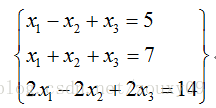
উপরের লিনিয়ার সমীকরণের জন্য, প্রথম এবং দ্বিতীয় সমীকরণের বিভিন্ন সমাধান রয়েছে, যখন দ্বিতীয় এবং তৃতীয় সমীকরণের ঠিক একই সমাধান রয়েছে। এই অর্থে, তৃতীয় সমীকরণটি "রিন্ডানডান্ট" কারণ এটি কোনও পরিমাণের তথ্য আনে না। এটি সরান এবং ফলস্বরূপ সমীকরণগুলি মূল সমীকরণগুলির মতো একই সমাধান। সমীকরণের সিস্টেম থেকে অপ্রয়োজনীয় সমীকরণগুলি সরিয়ে দেওয়ার জন্য, "ম্যাট্রিকের র্যাঙ্ক" ধারণাটি প্রাকৃতিকভাবে উদ্ভূত হয়েছিল।
মনে রাখবেন কীভাবে আমরা ম্যাট্রিককে ম্যানুয়ালি রেঙ্ক করি? ম্যাট্রিক্স এ এর র্যাঙ্কটি সন্ধান করার জন্য, আমরা ম্যাট্রিক্স প্রাথমিক ট্রান্সফর্মেশনের মাধ্যমে এটিকে ধাপে ধাপে ম্যাট্রিক্সে রূপান্তর করি the যদি ধাপে ধাপে ম্যাট্রিক্সে আর অ-শূন্য সারি থাকে, তবে A এর র্যাঙ্ক (A) আর এর সমান হয়। শারীরিক অর্থে, একটি ম্যাট্রিক্সের র্যাঙ্ক ম্যাট্রিক্সের সারি এবং কলামগুলির মধ্যে পারস্পরিক সম্পর্ককে পরিমাপ করে। যদি কোনও ম্যাট্রিক্সের সারি বা কলামগুলি লৈখিকভাবে স্বতন্ত্র থাকে তবে ম্যাট্রিক্স পূর্ণ র্যাঙ্ক, অর্থাত্ র্যাঙ্কটি সারি সংখ্যার সমান। উপরের লিনিয়ার সমীকরণগুলিতে ফিরে যান, কারণ লিনিয়ার সমীকরণগুলি ম্যাট্রিকেস দ্বারা বর্ণিত হতে পারে। কতগুলি দরকারী সমীকরণ রয়েছে তা রেঙ্কটি নির্দেশ করে। উপরোক্ত সমীকরণগুলিতে 3 টি সমীকরণ রয়েছে বাস্তবে, কেবল 2 টি কার্যকর এবং একটি অপ্রয়োজনীয়, সুতরাং সংশ্লিষ্ট ম্যাট্রিক্সের র্যাঙ্ক 2 হয়।
ঠিক আছে। যেহেতু র্যাঙ্ক পারস্পরিক সম্পর্ককে পরিমাপ করতে পারে তাই ম্যাট্রিক্স পারস্পরিক সম্পর্কের আসলে ম্যাট্রিক্সের সাথে কাঠামোগত তথ্য থাকে। যদি ম্যাট্রিক্সের সারিগুলির মধ্যে পারস্পরিক সম্পর্ক শক্তিশালী হয় তবে এর অর্থ হ'ল ম্যাট্রিক্সটি আসলে একটি নিম্ন-মাত্রিক লিনিয়ার উপ-স্পেসে প্রজেক্ট করা যেতে পারে, এটি কয়েকটি ভেক্টরের সাথে সম্পূর্ণরূপে প্রকাশ করা যেতে পারে, যা নিম্ন স্তরের। সুতরাং আমরা যা সংক্ষিপ্ত করছি তা হ'ল: ম্যাট্রিক্স যদি কাঠামোগত তথ্য যেমন চিত্র, ব্যবহারকারী-সুপারিশ সারণী ইত্যাদি প্রকাশ করে তবে এই ম্যাট্রিক্সের সারিগুলির মধ্যে একটি নির্দিষ্ট সম্পর্ক রয়েছে, তবে এই ম্যাট্রিক্সটি সাধারণত নিম্ন স্তরের হয়।
এক্স যদি এম সারি এবং এন কলাম সহ একটি সংখ্যাসূচক ম্যাট্রিক্স হয় এবং র্যাঙ্ক (এক্স) এক্স এর র্যাঙ্ক হয়, যদি র্যাঙ্ক (এক্স) এম এবং এন এর চেয়ে অনেক ছোট হয়, তবে আমরা এক্সকে নিম্ন র্যাঙ্কের ম্যাট্রিক্স বলি। নিম্ন-র্যাঙ্কের ম্যাট্রিক্সের প্রতিটি সারি বা কলামটি অন্যান্য সারি বা কলামগুলি লাইন করে প্রতিনিধিত্ব করতে পারে। দেখা যায় এটিতে প্রচুর অনর্থক তথ্য রয়েছে। এই অপ্রয়োজনীয় তথ্য দিয়ে, অনুপস্থিত তথ্য পুনরুদ্ধার করা যায়, এবং বৈশিষ্ট্যগুলিও ডেটা থেকে নেওয়া যেতে পারে।
ঠিক আছে, একটি নিম্ন পদ আছে, সুতরাং নিম্ন র্যাঙ্ককে সীমাবদ্ধ করা কেবলমাত্র র্যাঙ্ক (ডাব্লু) কে সীমাবদ্ধ করা হয় এই বিভাগে কার্নেলের আদর্শের সাথে এর কী সম্পর্ক আছে? তাদের সম্পর্ক L0 এবং L1 এর সম্পর্কের মতোই। যেহেতু র্যাঙ্ক () অব্যবহৃত নয়, এটি অপ্টিমাইজেশান সমস্যার সমাধান করা কঠিন, সুতরাং এটির আনুমানিকতার জন্য আমাদের এর উত্তল সন্ধান করতে হবে। হ্যাঁ, আপনি ঠিক বলেছেন, র্যাঙ্ক (ডাব্লু) এর উত্তল অনুকরণটি কার্নেলের আদর্শ W || ডাব্লু || * * ।
ঠিক আছে, এখানে আমার কিছু বলার নেই, কারণ আমিও এই জিনিসটির দিকে কিছুটা নজর রেখেছি, তাই আমি এটিতে সন্ধান করিনি। তবে আমি দেখতে পেলাম যে এই স্টাফটির জন্য এখনও অনেক আকর্ষণীয় অ্যাপ্লিকেশন রয়েছে, আসুন কয়েকটি সাধারণ কিছু নেওয়া যাক।
1) ম্যাট্রিক্স সমাপ্তি:
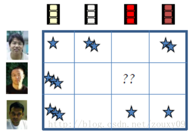
প্রথমে ম্যাট্রিক্স ফিলিংটি কোথায় ব্যবহৃত হয় সে সম্পর্কে আলোচনা করা যাক। একটি মূলধারার অ্যাপ্লিকেশনটি সুপারিশ সিস্টেমে রয়েছে। আমরা জানি যে তাদের historicalতিহাসিক রেকর্ড বিশ্লেষণ করে পরামর্শ দেওয়ার সিস্টেমগুলির জন্য ব্যবহারকারীদের সুপারিশ করার একটি উপায় রয়েছে। উদাহরণস্বরূপ, আমরা যখন কোনও সিনেমা দেখি, আমরা যদি এটি দেখতে পছন্দ করি তবে আমরা এটি 3 টি তার মতো একটি স্কোর দেব। তারপরে সিস্টেম, যেমন নেটফ্লিক্স এবং অন্যান্য সুপরিচিত ওয়েবসাইটগুলি প্রতিটি মুভিটির থিমটি ঠিক কী তা দেখার জন্য এই ডেটাগুলি বিশ্লেষণ করবে প্রত্যেকের জন্য, আপনি কী ধরণের সিনেমা পছন্দ করেন এবং তার পরে সংশ্লিষ্ট ব্যবহারকারীদের জন্য অনুরূপ চলচ্চিত্রের প্রস্তাব দিন। তবে একটি সমস্যা রয়েছে: আমাদের ওয়েবসাইটে প্রচুর ব্যবহারকারী এবং প্রচুর ভিডিও রয়েছে all সমস্ত ব্যবহারকারী কিছু সিনেমা দেখেনি, এবং সিনেমা দেখেছে এমন সমস্ত ব্যবহারকারী এটির রেট দেবে না। মনে করুন আমরা এই রেকর্ডগুলি বর্ণনা করতে যেমন একটি "ব্যবহারকারী-চলচ্চিত্র" ম্যাট্রিক্স ব্যবহার করি, যেমন নীচের চিত্রটি, আপনি দেখতে পারেন যে অনেকগুলি ফাঁকা জায়গা থাকবে। যদি এই ফাঁকা জায়গাগুলি বিদ্যমান থাকে তবে এই ম্যাট্রিক্সটি বিশ্লেষণ করা আমাদের পক্ষে কঠিন, সুতরাং বিশ্লেষণের আগে আমাদের সাধারণত এটি শেষ করা দরকার। একে ম্যাট্রিক্স ফিলও বলা হয়।
আপনি কিভাবে এটি পূরণ করবেন? কীভাবে আমাদের কিছুই নেই? প্রতিটি ফাঁকা জায়গায় থাকা তথ্যগুলিতে কি অন্যান্য বিদ্যমান তথ্য রয়েছে? যদি তা হয় তবে এটি কীভাবে উত্তোলন করা যায়? হ্যাঁ, এখানেই নিম্ন স্তরের খেলায় আসে। একে নিম্ন র্যাঙ্কের ম্যাট্রিক্স পুনর্গঠন সমস্যা বলা হয় এবং এটি নিম্নলিখিত মডেল দ্বারা প্রকাশ করা যেতে পারে: জ্ঞাত তথ্য একটি প্রদত্ত এম * এন ম্যাট্রিক্স এ the কিছু উপাদান যদি কোনও কারণে হারিয়ে যায় তবে আমরা কি অন্যান্য সারি এবং কলামগুলি ব্যবহার করতে পারি? উপাদানসমূহ, সেই উপাদানগুলি পুনরুদ্ধার করা হবে? অবশ্যই, অন্যান্য রেফারেন্স শর্ত ছাড়াই এই ডেটাগুলি নির্ধারণ করা কঠিন। তবে যদি আমরা A এর র্যাঙ্ক (A) << মি এবং র্যাঙ্ক (A) << n জানি তবে আমরা ম্যাট্রিক্সের সারি (কলাম) এর মধ্যে লিনিয়ার পারস্পরিক সম্পর্ক রেখে অনুপস্থিত উপাদানগুলি খুঁজে পেতে পারি। আপনি জিজ্ঞাসা করবেন, আমরা যে ম্যাট্রিক্সটি পুনরুদ্ধার করতে চাই তা নিম্ন র্যাঙ্কের কি তা ধরে নেওয়া কি যুক্তিসঙ্গত? প্রকৃতপক্ষে, এটি খুব যুক্তিসঙ্গত, উদাহরণস্বরূপ, কোনও চলচ্চিত্রের রেটিং ব্যবহারকারীরা এই মুভিটি রেটিং করে এমন অন্যান্য ব্যবহারকারীদের একটি রৈখিক সংমিশ্রণ। অতএব, নিম্ন-স্তরের পুনর্গঠন এমন ভিডিওগুলির জন্য ব্যবহারকারীদের পছন্দের মাত্রার পূর্বাভাস দিতে পারে যা মূল্যায়ন করা হয়নি। এভাবে ম্যাট্রিক্স পূরণ হচ্ছে।
2) Robust PCA:
প্রধান উপাদান বিশ্লেষণ, এই পদ্ধতিটি কার্যকরভাবে উপাত্তগুলির মধ্যে সর্বাধিক "প্রধান" উপাদান এবং কাঠামো সন্ধান করতে পারে, শব্দ এবং অপ্রয়োজনীয়তা সরিয়ে ফেলতে পারে, মূল জটিল ডেটাটিকে মাত্রিকতায় হ্রাস করতে পারে এবং জটিল তথ্যের পিছনে লুকানো সহজ কাঠামো প্রকাশ করতে পারে। আমরা জানি যে সহজতম পিসিএ পদ্ধতি হ'ল পিসিএ। লিনিয়ার বীজগণিতের দৃষ্টিকোণ থেকে, পিসিএর লক্ষ্য হ'ল ফলস্বরূপ ডেটা স্পেসটি নতুন করে সংজ্ঞায়িত করতে আরও একটি ঘাঁটি ব্যবহার করা। আশা করা যায় যে এই নতুন ফাউন্ডেশনের অধীনে মূল ডেটার মধ্যকার সম্পর্ক যতটা সম্ভব প্রকাশিত হতে পারে। এই মাত্রাটি সবচেয়ে গুরুত্বপূর্ণ "প্রধান উপাদান"। পিসিএর লক্ষ্য সর্বাধিক পরিমাণে অপ্রয়োজনীয়তা এবং শোরগোলের হস্তক্ষেপ দূর করার জন্য এই জাতীয় "অধ্যক্ষ" সন্ধান করা।
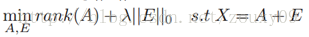
রবস্ট প্রিন্সিপাল কম্পোনেন্ট অ্যানালাইসিস (রোবস্ট পিসিএ) সমস্যাটিকে বিবেচনা করে: সাধারণত, আমাদের ডেটা ম্যাট্রিক্স এক্সটিতে কাঠামোগত তথ্য এবং গোলমাল থাকে। তারপরে আমরা এই ম্যাট্রিক্সকে দুটি ম্যাট্রিকগুলিতে দ্রবীভূত করতে পারি এবং সেগুলি যুক্ত করতে পারি, একটি হ'ল নিম্ন স্তরের (কারণ ভিতরে নির্দিষ্ট কাঠামোগত তথ্য রয়েছে, যার ফলে সারি বা কলামগুলির মধ্যে লিনিয়ার পারস্পরিক সম্পর্ক রয়েছে), এবং অন্যটি বিচ্ছিন্ন (শব্দের উপস্থিতির কারণে, গোলমাল বিরল), তবে শক্তিশালী প্রধান উপাদান বিশ্লেষণ নিম্নলিখিত অপ্টিমাইজেশন সমস্যা হিসাবে লেখা যেতে পারে:
ক্লাসিক পিসিএ সমস্যার মতো, শক্তিশালী পিসিএ হ'ল মূলত নিম্ন-মাত্রিক স্থানে ডেটার সেরা প্রক্ষেপণ সন্ধান করার সমস্যা। নিম্ন-র্যাঙ্কের ডেটা পর্যবেক্ষণ ম্যাট্রিক্স এক্সের জন্য, যদি এক্স এলোমেলো (স্পার্স) শব্দের দ্বারা প্রভাবিত হয়, এক্স এর নিম্ন র্যাঙ্কটি ধ্বংস হয়ে যাবে এবং এক্স পূর্ণ পদে পরিণত হবে। সুতরাং আমাদের নিম্ন-র্যাঙ্কের ম্যাট্রিক্স এবং এর আসল কাঠামোগুলি বিশিষ্ট শব্দের ম্যাট্রিক্সের যোগফলকে এক্স দ্রষ্টব্য করতে হবে। যখন একটি নিম্ন-র্যাঙ্কের ম্যাট্রিক্স পাওয়া যায়, তখন ডেটার প্রয়োজনীয় অপরিহার্য নিম্ন-মাত্রিক স্থানটি পাওয়া যায়। তাহলে পিসিএর সাথে কেন সেখানে শক্ত শক্ত পিসিএ আছে? শক্ত কোথায়? কারণ পিসিএ ধরে নিয়েছে যে আমাদের ডেটার আওয়াজ গাউসিয়ান, বড় শব্দ বা গুরুতর আউটলিয়ারদের জন্য, পিসিএ এতে ক্ষতিগ্রস্থ হবে, যার ফলে এটি ক্ষতিগ্রস্থ হবে। এই ধারণাটি রোবস্ট পিসিএর জন্য বিদ্যমান নেই। এটি কেবল ধরেই নিয়েছে যে এর শব্দ নির্বিশেষে এর শব্দটি বিরল sp
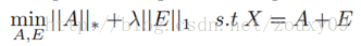
যেহেতু র্যাঙ্ক এবং এল0 নীতিগুলির অপ্টিমাইজেশনে নন-উত্তল এবং নন-মসৃণ বৈশিষ্ট্য রয়েছে, তাই আমরা সাধারণত এটিকে নিম্নোক্ত শিথিল উত্তল উত্তোলন সমস্যা সমাধানের জন্য রূপান্তর করি:
এর অ্যাপ্লিকেশন সম্পর্কে কথা বলা যাক। একই মুখের একাধিক চিত্র বিবেচনা করে যদি প্রতিটি মুখের চিত্রটি একটি সারি ভেক্টর হিসাবে বিবেচনা করা হয় এবং এই ভেক্টরগুলি একটি ম্যাট্রিক্সে গঠিত হয়, তবে এটি নিশ্চিত হতে পারে যে, তাত্ত্বিকভাবে, এই ম্যাট্রিক্সটি নিম্ন স্তরের হওয়া উচিত। তবে, প্রকৃত ক্রিয়াকলাপে, প্রতিটি চিত্র কিছু পরিমাণে প্রভাবিত হবে, যেমন অবসান, গোলমাল, আলো পরিবর্তন, অনুবাদ ইত্যাদি etc. এই হস্তক্ষেপ কারণগুলির প্রভাবটি একটি শব্দ ম্যাট্রিক্সের প্রভাব হিসাবে দেখা যায়। তাই আমরা একাধিক বিভিন্ন ক্ষেত্রে আমাদের একই মুখের ছবিগুলি লম্বা করতে পারি এবং তারপরে এগুলি একটি ম্যাট্রিক্সে সাজিয়ে তুলি clean পরিষ্কার মুখের চিত্র পেতে (নিম্ন র্যাঙ্কের জন্য) এই ম্যাট্রিক্সকে কম র্যাঙ্ক এবং বিরল পচন সহ বিশিষ্ট করুন ম্যাট্রিক্স এবং শব্দের ম্যাট্রিক্স (স্পার্স ম্যাট্রিক্স), যেমন আলোক, আবরণ ইত্যাদি এই উদ্দেশ্য হিসাবে, আপনি জানেন।
3) Background modeling::
ব্যাকগ্রাউন্ড মডেলিংয়ের সহজতম ক্ষেত্রে হ'ল স্থির ক্যামেরায় নেওয়া ভিডিও থেকে ব্যাকগ্রাউন্ড এবং সম্মুখভাগ পৃথক করা। আমরা ভিডিও চিত্র সিকোয়েন্সের প্রতিটি ফ্রেমের পিক্সেল মানগুলি একটি কলাম ভেক্টরে টানছি এবং তারপরে একাধিক ফ্রেম অর্থাৎ একাধিক কলাম ভেক্টর একটি পর্যবেক্ষণ ম্যাট্রিক্স গঠন করে। যেহেতু ব্যাকগ্রাউন্ড তুলনামূলকভাবে স্থিতিশীল এবং চিত্র সিকোয়েন্সের ফ্রেমের মধ্যে দুর্দান্ত মিল রয়েছে, কেবলমাত্র ব্যাকগ্রাউন্ড পিক্সেলের সমন্বিত ম্যাট্রিক্সের নিম্নমানের বৈশিষ্ট্য রয়েছে the একই সাথে, কারণ সম্মুখভাগটি একটি চলমান বস্তু এবং পিক্সেলের অনুপাত কম, अग्रভূমি পিক্সেলগুলি সমন্বিত। ম্যাট্রিক্স বিরল। ভিডিও পর্যবেক্ষণ ম্যাট্রিক্স এই দুটি চরিত্রগত ম্যাট্রিক্সের সুপারপজিশন Therefore সুতরাং, এটি বলা যেতে পারে যে ভিডিও ব্যাকগ্রাউন্ড মডেলিংয়ের প্রক্রিয়াটি নিম্ন-স্তরের ম্যাট্রিক্স পুনরুদ্ধারের প্রক্রিয়া।
4) Transform Invariant Low Rank Texture (TILT):
পূর্ববর্তী বিভাগে প্রবর্তিত চিত্রগুলির জন্য নিম্ন-স্তরের আনুমানিক অ্যালগরিদম কেবল চিত্রের নমুনাগুলির মধ্যে পিক্সেলের সাদৃশ্য বিবেচনা করে তবে দ্বি-মাত্রিক পিক্সেল সেট হিসাবে চিত্রের নিয়মিততাটিকে বিবেচনায় নেয় না। প্রকৃতপক্ষে, কোনও ঘূর্ণনবিহীন চিত্রের জন্য, চিত্রটির প্রতিসাম্য এবং স্ব-মিলের কারণে, আমরা এটিকে শব্দের সাথে নিম্ন-স্তরের ম্যাট্রিক্স হিসাবে ভাবতে পারি। চিত্রটি যখন স্বাভাবিক থেকে ঘোরানো হয় তখন চিত্রটির প্রতিসাম্য এবং নিয়মিততা নষ্ট হয়ে যায়, অর্থাৎ, প্রতিটি সারিতে পিক্সেলের মধ্যে লিনিয়ার পারস্পরিক সম্পর্ক নষ্ট হয়ে যায়, সুতরাং ম্যাট্রিক্সের র্যাঙ্কটি বৃদ্ধি পাবে।
ট্রান্সফর্ম ইনভেরিয়েন্ট লো-র্যাঙ্ক টেক্সচার (টিআইএলটি) হ'ল একটি নিম্ন-র্যাঙ্কের টেক্সচার পুনরুদ্ধার অ্যালগরিদম যা নিম্ন র্যাঙ্ক এবং শব্দ শূন্যতার ব্যবহার করে। এর ধারণাটি হ'ল অনুভূমিক, উল্লম্ব এবং প্রতিসম বৈশিষ্ট্যযুক্ত জ্যামিতিক রূপান্তর-এর মাধ্যমে নিয়মিত অঞ্চলে ডি দ্বারা প্রতিনিধিত্ব করা চিত্রের অঞ্চলটি সংশোধন করা These এই বৈশিষ্ট্যগুলি নিম্ন স্তরের দ্বারা চিহ্নিত করা যায়।
অনেকগুলি নিম্ন-স্তরের অ্যাপ্লিকেশন রয়েছে you আপনি যদি আগ্রহী হন তবে আরও কিছু জানতে আপনি কিছু তথ্য সন্ধান করতে পারেন।
Fourth, the choice of regularization parameters
এখন আসুন ফিরে আসুন এবং আমাদের উদ্দেশ্য ফাংশনটি দেখুন:
ক্ষতি এবং নিয়মের শর্তাদি ছাড়াও, একটি প্যারামিটারও রয়েছে λ এটির হাইপার-প্যারামিটার নামে একটি স্বভাবের নামও রয়েছে। আপনি একা এটি দেখতে চান না, এটি খুব গুরুত্বপূর্ণ। যখন এর মান খুব বড় হয়, এটি আমাদের মডেলটির কর্মক্ষমতা নির্ধারণ করবে, যা মডেলের জীবন এবং মৃত্যুর সাথে সম্পর্কিত। এটি প্রধানত ক্ষতির দুটি শর্ত এবং নিয়মিত শর্তগুলিতে ভারসাম্য বজায় রাখে The বৃহত্তর λ এর অর্থ হল নিয়মিত শর্তগুলি মডেল প্রশিক্ষণের ত্রুটির চেয়ে বেশি গুরুত্বপূর্ণ, আমরা আমাদের মডেলটিকে আমাদের ডেটা ফিট করার চেয়ে বেশি সন্তুষ্ট করতে চাই। আমরা Ω (ডাব্লু) এর বৈশিষ্ট্যকে সীমাবদ্ধ করি। এবং বিপরীত। একটি চরম ক্ষেত্রে উদাহরণস্বরূপ, যখন, = 0 হয়, তখন কোনও পরবর্তী শব্দ থাকে না function ব্যয়ের ফাংশনটি হ্রাস করা প্রথম পদটির উপর নির্ভর করে, অর্থাত্ আউটপুট এবং প্রত্যাশিত আউটপুটটির মধ্যে পার্থক্য হ্রাস করার জন্য পূর্ণ শক্তি ব্যবহৃত হয় the পার্থক্যটি সবচেয়ে ছোট কখন? অবশ্যই এটি আমাদের ফাংশন বা বক্ররেখা যা সমস্ত পয়েন্টের মধ্য দিয়ে যেতে পারে এই সময়ে, ত্রুটি 0 এর কাছাকাছি, যা অত্যধিক মানানসই। এটি জটিলভাবে এই সমস্ত নমুনা উপস্থাপন বা মুখস্ত করতে পারে, তবে নতুন নমুনার জন্য সাধারণীকরণের ক্ষমতা যথেষ্ট নয়। সর্বোপরি, নতুন নমুনা প্রশিক্ষণের নমুনা থেকে আলাদা হবে।
তাহলে আমাদের আসলে কী দরকার? আমরা আশা করি যে আমাদের মডেলটি আমাদের ডেটা মাপসই করতে পারে এবং আমাদের সীমাবদ্ধ করে এমন বৈশিষ্ট্য থাকতে পারে। কেবলমাত্র উভয়েরই নিখুঁত সংমিশ্রণটি আমাদের কাজটিতে আমাদের মডেলটিকে শক্তিশালীভাবে সম্পাদন করতে পারে। সুতরাং কিভাবে এটি সন্তুষ্ট করা খুব গুরুত্বপূর্ণ। এই মুহুর্তে, প্রত্যেকের গভীর ধারণা থাকতে পারে। মনে রাখবেন যে আপনি প্রচুর কাগজ প্রজনন করেছেন এবং তারপরে পুনরুত্পাদন কোডের যথার্থতা তত বেশি ছিল না যতটা কাগজটি বলেছিল, তার চেয়েও খারাপ। এই সময়ে, আপনি সন্দেহ করবেন যে এটি থিসিসের সমস্যা কিনা বা আপনার উপলব্ধির সমস্যা? আসলে, এই দুটি প্রশ্ন ছাড়াও, আমাদের আরও একটি প্রশ্ন সম্পর্কে গভীরভাবে চিন্তা করা প্রয়োজন: কাগজে প্রস্তাবিত মডেলটির হাইপার-প্যারামিটারগুলি রয়েছে? কাগজটি কি তাদের পরীক্ষামূলক মান দিয়েছে? অভিজ্ঞতা অভিজ্ঞতা বা ক্রস-বৈধ মূল্য? এই সমস্যাটি এড়াতে পারা যায় না, কারণ প্রায় কোনও সমস্যা বা মডেলটিতে হাইপার-প্যারামিটার থাকবে তবে কখনও কখনও এটি লুকানো থাকে এবং আপনি এটি দেখতে পারবেন না, তবে একবার আপনি যদি এটি আবিষ্কার করেন যে এটি প্রমাণ করে যে আপনার ভাগ্য রয়েছে, তবে চেষ্টা করুন এগিয়ে যান এবং এটি সংশোধন করুন, "অলৌকিক ঘটনা" ঘটতে পারে।
ঠিক আছে, নিজেই প্রশ্নটিতে ফিরে আসুন। পরামিতিটি বেছে নেওয়ার ক্ষেত্রে আমাদের লক্ষ্য কী? আমরা আশা করি প্রশিক্ষণের ত্রুটি এবং মডেলটির সাধারণীকরণের ক্ষমতা শক্তিশালী। এই মুহুর্তে, আপনি এখনও এটি প্রতিফলিত করতে পারেন, এর অর্থ এই নয় যে আমাদের সাধারণীকরণের পারফরম্যান্সটি আমাদের প্যারামিটারের ফাংশন function? তাহলে আমরা কেন ল্যাম্বডাকে বেছে নেব যা অপ্টিমাইজড সেট অনুসারে সাধারণকরণের কার্য সম্পাদনকে সর্বাধিকতর করতে পারে? ওহ, আপনাকে জানাতে দুঃখিত, কারণ সাধারণীকরণের কার্য সম্পাদন of এর কোনও সাধারণ কাজ নয়! এটির অনেক স্থানীয় সর্বাধিক! এবং এর অনুসন্ধানের স্থানটি বিশাল। অতএব, আপনি যখন প্যারামিটারগুলি নির্ধারণ করবেন তখন একটি হ'ল প্রচুর অভিজ্ঞতার মানগুলি চেষ্টা করা উচিত যা এই ক্ষেত্রগুলিতে স্ক্র্যাচিং এবং রোলিং করছে এমন মাস্টারদের সাথে অতুলনীয়। অবশ্যই, কিছু মডেলগুলির জন্য, মাস্টাররা আমাদের জন্য কিছু টিউনিংয়ের অভিজ্ঞতাও সংকলন করেছিলেন। উদাহরণস্বরূপ, ভাই হিন্টনের প্রশিক্ষণ সীমাবদ্ধ বল্টজম্যান মেশিনগুলি সম্পর্কিত একটি ব্যবহারিক গাইড। আরেকটি পদ্ধতি হ'ল আমাদের মডেল বিশ্লেষণ করে চয়ন করা। এটা কিভাবে করবেন? প্রশিক্ষণের ঠিক আগে, এই সময়ে ক্ষতির মেয়াদটির মূল্য কী? Ω (ডাব্লু) এর মান কত? তারপরে আমরা তাদের লম্বা তাদের অনুপাতের জন্য নির্ধারণ করি This এই হিউরিস্টিক পদ্ধতিটি আমাদের অনুসন্ধানের স্থান হ্রাস করবে। আর একটি সর্বাধিক সাধারণ পদ্ধতি হ'ল ক্রস-বৈধকরণ ক্রস বৈধতা। প্রথমে আমাদের প্রশিক্ষণ ডাটাবেসটিকে কয়েকটি অংশে বিভক্ত করুন, তারপরে প্রশিক্ষণ সেট হিসাবে একটি অংশ এবং পরীক্ষার সেট হিসাবে একটি অংশ নিন এবং তারপরে এন মডেলগুলি প্রশিক্ষণের জন্য এই প্রশিক্ষণ সেটটি ব্যবহার করতে বিভিন্ন ল্যাম্বডাস বেছে নিন এবং তারপরে আমাদের মডেল পরীক্ষার জন্য এই পরীক্ষার সেটটি ব্যবহার করুন, এন নিন মডেলটিতে পরীক্ষার ত্রুটির সাথে ন্যূনতম λ আমাদের চূড়ান্ত হিসাবে নেওয়া হয় λ যদি আমাদের মডেলটি দীর্ঘ সময়ে প্রশিক্ষণপ্রাপ্ত হয় তবে এটি স্পষ্ট যে আমরা কেবলমাত্র খুব কম পরীক্ষা করতে পারি limited সীমিত সময়ে। উদাহরণস্বরূপ, ধরুন আমাদের মডেলটিকে 1 দিনের জন্য প্রশিক্ষণ দেওয়া দরকার যা গভীর শিক্ষার ক্ষেত্রে সাধারণ, এবং তারপরে আমাদের এক সপ্তাহ থাকে, তবে আমরা কেবল 7 টি আলাদা ল্যাম্বডা পরীক্ষা করতে পারি। এটি আপনাকে সেরাটির সাথে মিলিত হতে দেয় which যা শেষ জীবনে জমা হওয়া আশীর্বাদ। কোন উপায় আছে? দুটি ধরণের রয়েছে: একটি হ'ল আরও 7 টি নির্ভরযোগ্য ল্যাম্বডা পরীক্ষা করার চেষ্টা করা, বা ল্যাম্বদার অনুসন্ধানের স্থানটি যতটা সম্ভব বিস্তৃত করা, তাই ল্যাম্বদার জন্য অনুসন্ধানের জায়গার পছন্দটি সাধারণত -10 থেকে 10 এর মধ্যে দু'টির শক্তি বা কিছু। যাইহোক, এই পদ্ধতিটি এখনও নির্ভরযোগ্য নয় এবং সর্বোত্তম পদ্ধতিটি হল আমাদের মডেল প্রশিক্ষণের জন্য প্রয়োজনীয় সময়কে হ্রাস করা। উদাহরণস্বরূপ, ধরুন আমরা আমাদের মডেল প্রশিক্ষণকে অনুকূলিত করি যাতে আমাদের প্রশিক্ষণের সময়টি ২ ঘন্টার মধ্যে কমে যায়। তারপরে আমরা সপ্তাহে week * ২৪/২ = ৮৪ বার মডেলটিকে প্রশিক্ষণ দিতে পারি, অর্থাৎ আমরা ৮৪ টি ল্যাম্বডাসের মধ্যে সেরা ল্যাম্বডাকে খুঁজে পেতে পারি। এটি আপনাকে সবচেয়ে ভাল ল্যাম্বডায় দেখা করার সম্ভাবনা তৈরি করে। এ কারণেই আমাদের একটি অ্যালগরিদম চয়ন করতে হবে যা রূপান্তর করার জন্য দ্রুত, মডেল প্রশিক্ষণের জন্য কেন জিপিইউ, মাল্টি-কোর, ক্লাস্টার ইত্যাদি ব্যবহার করতে পারে এবং শক্তিশালী কম্পিউটার সংস্থানযুক্ত শিল্প কেন এমন অনেক কিছু করতে পারে যা একাডেমিয়া করতে পারে না (অবশ্যই) বড় ডেটাও একটি কারণ)।
"টিউনিং" এর মাস্টার হওয়ার চেষ্টা করুন! আমি আশা করি আপনারা সবাই "সেরা জিনসেং পান!"
ভি। রেফারেন্স
[1] http://fastML.com/large-scale-l1-feature-selection-with-vowpal-wabbit/
[২] http://www.stat.purdue.edu/~vishy/introml/notes/Optimization.pdf
[3] http://www.stanford.edu/~boyd/cvxbook/bv_cvxbook.pdf
[৫] http://nm.mathforcolleg.com/mws/gen/04sle/mws_gen_sle_spe_adequacy.pdf
In the previous blog post , we talked about the L0, L1, and L2 norms. In this post , we talk about the kernel norms and rule parameter selection. Knowledge is limited. The following are my simple ideas. If there are errors in understanding, I hope everyone can correct them. Thank you.
Third, the nuclear norm
The kernel norm || W || * refers to the sum of the singular values of the matrix, which is called Nuclear Norm in English. Compared to the hot L1 and L2 above, everyone may be unfamiliar. So what is it used for? Domineering debut: Constrained Low-Rank. OK, OK, then we need to know what Low-Rank is? What is it for?
Let's first recall what the "rank" is in linear algebra. Take a simple example:
For the above linear equations, the first and second equations have different solutions, while the second and third equations have exactly the same solution. In this sense, the third equation is "redundant" because it does not bring any amount of information. Remove it, and the resulting equations are the same solution as the original equations. In order to remove redundant equations from the system of equations, the concept of "rank of matrices" was naturally derived.
Remember how we manually rank the matrices? In order to find the rank of matrix A, we transform A into a stepwise matrix through matrix elementary transformation. If the stepwise matrix has r non-zero rows, then the rank rank (A) of A is equal to r. In a physical sense, the rank of a matrix measures the correlation between the rows and columns of the matrix. If the rows or columns of a matrix are linearly independent, the matrix is full rank, that is, the rank is equal to the number of rows. Back to the linear equations above, because linear equations can be described by matrices. Rank indicates how many useful equations there are. The above equations have 3 equations. In fact, only 2 are useful, and one is redundant, so the rank of the corresponding matrix is 2.
OK. Since rank can measure correlation, matrix correlation actually has structural information with matrix. If the correlation between the rows of the matrix is strong, it means that the matrix can actually be projected into a lower-dimensional linear subspace, that is, it can be fully expressed with a few vectors, which is low rank. So what we summarize is: if the matrix expresses structural information, such as images, user-recommendation tables, etc., then there is a certain correlation between the rows of this matrix, then this matrix is generally low rank.
If X is a numerical matrix with m rows and n columns, and rank (X) is the rank of X, if rank (X) is much smaller than m and n, then we call X a low rank matrix. Each row or column of a low-rank matrix can be linearly represented by other rows or columns. It can be seen that it contains a lot of redundant information. With this redundant information, the missing data can be recovered, and features can also be extracted from the data.
Okay, there is a low rank, so constraining the low rank is only constraining rank (w). What does it have to do with the kernel norm in this section? Their relationship is the same as the relationship between L0 and L1. Because rank () is non-convex, it is difficult to solve in the optimization problem, so we need to find its convex approximation to approximate it. Yes, you are right, the convex approximation of rank (w) is the kernel norm || W || * * .
Well, here I have nothing to say, because I also looked at this thing a bit, so I haven't looked into it. But I found that there are still many interesting applications for this stuff, let's take a few typical ones.
1) Matrix Completion:
Let's first talk about where matrix filling is used. A mainstream application is in recommendation systems. We know that there is a way for recommendation systems to recommend users by analyzing their historical records. For example, when we watch a movie, if we like to watch it, we will give it a score, such as 3 stars. Then the system, such as Netflix and other well-known websites, will analyze these data to see what the theme of each movie is exactly? For everyone, what kind of movies do you like, and then recommend similar movies to the corresponding users. But there is a problem: there are a lot of users and a lot of videos on our website. Not all users have seen some movies, and not all users who have seen a movie will rate it. Suppose we use a "user-movie" matrix to describe these records, such as the following figure, you can see that there will be a lot of blank spaces. If these blank spaces exist, it is difficult for us to analyze this matrix, so we generally need to complete it before analysis. Also called matrix fill.
So how do you fill it out? How can we have nothing out of nothing? Does the information in each blank place contain other existing information? If so, how to extract it? Yeah, this is where low rank comes into play. This is called the low-rank matrix reconstruction problem, and it can be expressed by the following model: Known data is a given m * n matrix A. If some of the elements are lost for some reason, can we use other rows and columns? Elements, will those elements be restored? Of course, it is difficult to determine these data without other reference conditions. But if we know the rank rank (A) << m and rank (A) << n of A, then we can find the missing elements by linear correlation between the rows (columns) of the matrix. You would ask, is it reasonable to assume that the matrix we want to recover is low rank? In fact, it is very reasonable, for example, a user rating a movie is a linear combination of other users rating this movie. Therefore, low-rank reconstruction can predict the degree of user preference for videos that have not been evaluated. Thus filling the matrix.
2) Robust PCA:
Principal component analysis, this method can effectively find the most "main" elements and structures in the data, remove noise and redundancy, reduce the original complex data to dimensionality, and reveal the simple structure hidden behind the complex data. We know that the simplest PCA method is PCA. From a linear algebra perspective, the goal of PCA is to use another set of bases to redefine the resulting data space. It is hoped that under this new foundation, the relationship between the original data can be revealed as much as possible. This dimension is the most important "principal element". The goal of PCA is to find such "principals" to remove the interference of redundancy and noise to the greatest extent.
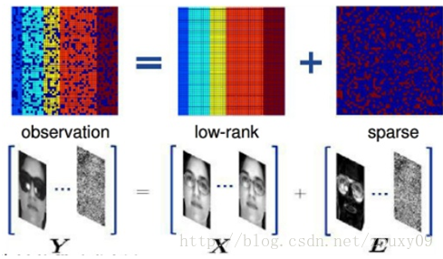
Robust Principal Component Analysis (Robust PCA) considers the problem: Generally, our data matrix X will contain structural information and noise. Then we can decompose this matrix into two matrices and add them, one is low rank (because there is certain structural information inside, resulting in linear correlation between rows or columns), and the other is sparse (due to the presence of noise, the Noise is sparse), then robust principal component analysis can be written as the following optimization problem:
Like the classic PCA problem, robust PCA is essentially the problem of finding the best projection of data on a low-dimensional space. For the low-rank data observation matrix X, if X is affected by random (sparse) noise, the low rank of X will be destroyed, making X become full rank. So we need to decompose X into the sum of the low-rank matrix and the sparse noise matrix containing its real structure. When a low-rank matrix is found, the essential low-dimensional space of the data is actually found. So with PCA, why is there Robust PCA? Where is Robust? Because PCA assumes that the noise of our data is Gaussian, for large noise or severe outliers, PCA will be affected by it, causing it to malfunction. This assumption does not exist for Robust PCA. It just assumes that its noise is sparse, regardless of its strength.
Because rank and L0 norms have non-convex and non-smooth characteristics in optimization, we generally convert it to solve the following relaxed convex optimization problem:
Let's talk about applications. Considering multiple images of the same face, if each face image is regarded as a row vector and these vectors are formed into a matrix, then it can be sure that, in theory, this matrix should be low rank. However, in actual operation, each image will be affected to some extent, such as occlusion, noise, lighting changes, translation, etc. The effect of these interference factors can be seen as the effect of a noise matrix. So we can lengthen the pictures of our same face in multiple different cases, and then arrange them into a matrix. Decompose this matrix with low rank and sparse decomposition to get a clean face image (low rank Matrix) and noise matrix (sparse matrix), such as lighting, occlusion, etc. As for the purpose of this, you know.
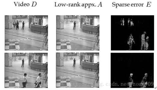
3) Background modeling:
The simplest case of background modeling is to separate the background and foreground from the video taken by the fixed camera. We pull the pixel values of each frame of the video image sequence into a column vector, and then multiple frames, that is, multiple column vectors form an observation matrix. Because the background is relatively stable and there is great similarity between the frames of the image sequence, the matrix consisting only of background pixels has a low rank characteristic. At the same time, because the foreground is a moving object and the proportion of pixels is low, the foreground pixels are composed. The matrix is sparse. The video observation matrix is the superposition of these two characteristic matrices. Therefore, it can be said that the process of video background modeling is the process of low-rank matrix recovery.
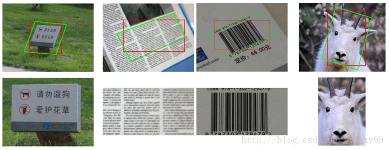
4) Transform Invariant Low Rank Texture (TILT):
The low-rank approximation algorithm for images introduced in the previous section only considers the similarity of pixels between image samples, but does not take into account the regularity of the image as a two-dimensional pixel set. In fact, for an image without rotation, due to the symmetry and self-similarity of the image, we can think of it as a low-rank matrix with noise. When the image is rotated from the normal, the symmetry and regularity of the image will be destroyed, that is, the linear correlation between the pixels in each row is destroyed, so the rank of the matrix will increase.
Transform Invariant Low-rank Textures (TILT) is a low-rank texture restoration algorithm that uses low rank and noise sparsity. Its idea is to correct the image area represented by D to a regular area through geometric transformation τ, such as having horizontal, vertical, and symmetrical characteristics. These characteristics can be characterized by low rank.
There are many low-rank applications. If you are interested, you can find some information to learn more.
Fourth, the choice of regularization parameters
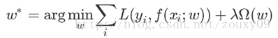
Now let's go back and look at our objective function:
In addition to the loss and rule terms, there is also a parameter λ. It also has a domineering name called hyper-parameters. You don't want to look at it alone, it is very important. When its value is very large, it will determine the performance of our model, which is related to the life and death of the model. It mainly balances the two terms of loss and regular terms. The larger λ means that the regular terms are more important than the model training error, that is, we want our model to satisfy more than to fit our data. We constrain the characteristic of Ω (w). vice versa. For an extreme case, for example, when λ = 0, there is no latter term. The minimization of the cost function depends on the first term, that is, the full force is used to minimize the difference between the output and the expected output. When is the difference the smallest? It is our function or curve that can pass through all the points. At this time, the error is close to 0, which is overfitting. It can complexly represent or memorize all these samples, but the generalization ability for a new sample is not enough. After all, the new sample will be different from the training sample.
So what do we really need? We hope that our model can fit our data and have the characteristics that we constrain it. Only the perfect combination of both of them can make our model perform powerfully on our task. So how to please it is very important. At this point, everyone may have a deep understanding. Remember that you reproduced a lot of papers, and then the accuracy of the reproduced code was not as high as the paper said, even worse. At this time, you will doubt whether it is the problem of the thesis or the problem of your realization? In fact, in addition to these two questions, we need to think deeply about another question: Does the model proposed in the paper have hyper-parameters? Did the paper give their experimental values? Empirical value or cross-validated value? This problem cannot be escaped, because almost any problem or model will have hyper-parameters, but sometimes it is hidden and you can't see it, but once you find out that it proves that you have a fate, then try Go ahead and modify it, there may be "miracles" happen.
OK, back to the question itself. What is our goal in choosing the parameter λ? We hope that the training error and generalization ability of the model are strong. At this time, you may still reflect it, does this not mean that our generalization performance is a function of our parameter? Then why do we choose the lambda that can maximize the generalization performance according to the optimized set? Oh, sorry to tell you that, because generalization performance is not a simple function of λ! It has many local maximums! And its search space is huge. Therefore, when you determine the parameters, one is to try a lot of experience values, which is incomparable with those masters who are scratching and rolling in this field. Of course, for some models, the masters also compiled some tuning experience for us. For example, Brother Hinton's A Practical Guide to Training Restricted Boltzmann Machines and so on. Another method is to choose by analyzing our model. How to do it? Just before training, what is the value of the loss term at this time? What is the value of Ω (w)? Then we determine our lambda for their proportion. This heuristic method will reduce our search space. Another most common method is cross-validation Cross validated. First divide our training database into several parts, then take a part as the training set and a part as the test set, and then choose different lambdas to use this training set to train N models, and then use this test set to test our model, take N The minimum λ corresponding to the test error in the model is taken as our final λ. If our model is trained for a long time at a time, it is obvious that we can only test very little λ in a limited time. For example, suppose our model needs to be trained for 1 day, which is commonplace in deep learning, and then we have one week, then we can only test 7 different lambdas. This allows you to meet the best λ, which is the blessing accumulated in the last life. Is there any way? There are two types: one is to try to test 7 more reliable lambdas, or to make the search space of lambda as wide as possible, so the choice of the search space for lambda is generally the power of two, from -10 to 10 What. However, this method is still not reliable, and the best method is to minimize the time required for our model training. For example, suppose we optimize our model training so that our training time is reduced to 2 hours. Then we can train the model 7 * 24/2 = 84 times a week, that is, we can find the best lambda among 84 lambdas. This makes you most likely to meet the best lambda. This is why we have to choose an algorithm that is fast to converge, why use GPU, multi-core, cluster, etc. for model training, and why the industry with powerful computer resources can do many things that academia cannot do (of course) Big data is also a reason).
Strive to be a master of "Tuning"! I wish you all "get the best ginseng!"
0 comments:
Post a Comment