This series of machine learning algorithms and Python practice is mainly based on the book "Machine Learning in Action " . Because I want to learn Python and then I want to learn more about some machine learning algorithms, I want to implement several more commonly used machine learning algorithms through Python. I happened to meet this samely-oriented book, so I used the process of this book to learn.
In this section, we mainly review the SVM system and implement it through Python. Since there is so much content, here are three blog posts. The first one talks about the basics of SVM, the second one talks about advanced, which mainly straightens the entire knowledge chain of SVM, and the third one introduces the implementation of Python. SVM has a lot of very good blog posts, you can refer to the references and recommended readings listed in this article. In this article, the positioning is to straighten out the overall knowledge chain of the integrated SVM, so it will not involve the derivation of details. There are many good deductions and books on the Internet, and you can refer to them.
table of Contents
I. Introduction
Second, linearly separable SVM and hard interval maximization
Third, the dual optimization problem
3.1 Duality
3.2 Dual Problem of SVM Optimization
Fourth, relaxation vector and soft interval maximization
Five, the kernel function
Six, multi-class classification SVM
6.1, "One-to-many" method
6.2. "One to one" method
Analysis of KKT conditions
Eight, SMO implementation of SMO algorithm
8.1 Coordinate descent algorithm
8.2, SMO algorithm principle
8.3.Python implementation of SMO algorithm
References and recommended reading
Five, the kernel function
If our normal sample distribution is shown on the left side of the figure below, the reason why it is normal means that it is not linearly inseparable due to some stubborn outliers as mentioned above. It is really linear and indivisible. The distribution of the sample itself is like this. If you also pull out a linear classification boundary through the relaxation variable like the sample, it is obvious that this classification surface will be very bad. then what should we do? SVM is effective for linearly separable data. What are some good strategies for inseparable? It's time for the kernel trick.
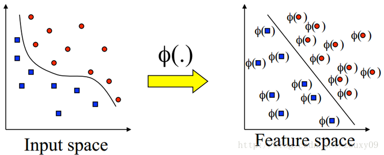
As shown on the right of the figure above, if we can transform our original sample points to another feature space, which is linearly separable on this feature space, then the above SVM can easily work. That is, for inseparable data, we now need to do two things:
1) First use a non-linear map Φ ( x ) to transform all the original data x to another feature space, in which the samples become linearly separable
2) Then use SVM in the feature space for learning classification.
Well, there is nothing to say about the second job, as before. Who will do the first heavy work? How do we know which transformation can map our data to be linearly separable? The data dimension is so large that we can't see it. In addition, will this transformation complicate the optimization of the second step and make it more computationally expensive? For the first problem, there is a well-known cover theorem: Projecting a complex pattern classification problem nonlinearly into a high-dimensional space will be more likely to be linearly separable than a low-dimensional space. OK, that's easy, we have to find a mapping where all the samples are mapped to a higher dimensional space. Sorry, it is actually very difficult to find this mapping function. However, the support vector machine does not directly find and calculate this complex non-linear transformation, but rather intelligently implements this transformation indirectly through a clever circuitous method. It is the kernel function, which not only has this super power, but also does not increase the computational cost of the best of both worlds. We can look back at the optimization problem of the SVM above:
It can be seen that for the use of sample x , it is only necessary to calculate the inner product of the i-th and j-th samples.
For the classification decision function, the inner product of two samples is also calculated. That is, both training the SVM and using the SVM use the inner product between samples, and only the inner product is used. Then if we can find a way to calculate the value of the inner product of two samples mapped to a high-dimensional space. The kernel function accomplishes this great mission:
K ( x i , x j ) = Φ ( x i ) T Φ ( x j )
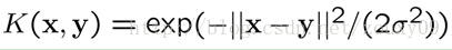
That is , the inner product Φ ( x i ) T Φ ( x j ) of the high-dimensional space corresponding to the two samples x i and x j is calculated by a kernel function K ( x i , x j ).. Without knowing who this transformation Φ ( x ) is. And the calculation of this kernel function is very simple. The radial basis RBF function is commonly used:
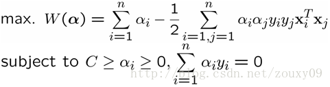
At this point, our optimized duality problem becomes:
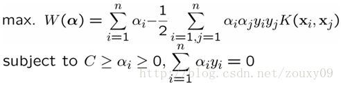
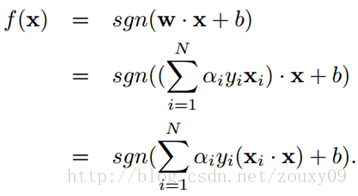
The only difference from the previous optimization problem is that the inner product of the samples needs to be replaced with a kernel function. There is no difference in the optimization process. And the decision function becomes:
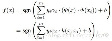
That is, the new sample x and all our training samples can be used to calculate the kernel function. It should be noted that because the Lagrange factor α i of most samples is 0, in fact, we only need to calculate the kernel function of a small number of training samples and new samples, and then sum and take the sign to complete the new Here comes the classification of sample x . The decision process of support vector machine can also be regarded as a similarity comparison process. First, the input samples are compared with a series of template samples. The template samples are the support vectors determined by the training process, and the similarity measure used is the kernel function. The score after the sample is compared with each support vector is weighted and summed, and the weight is the performance of the coefficient α i and the class label of each support vector obtained during training . Finally, the decision is made based on the weighted sum. And using different kernel functions is equivalent to using different methods of measuring similarity.
From a computational point of view, no matter how high the spatial dimension of the Φ ( x ) transformation is, even an infinite dimension (the function is infinite dimension), the solution of the linear support vector machine in this space can be performed by the kernel function in the original space. The calculation in the high-dimensional space can be avoided, and the complexity of calculating the kernel function and the complexity of calculating the inner product of the original sample are not substantially increased.
Here, I can't help but sigh. Why does the "vector" SVM always need to be calculated in the form of an inner product? Why does "coincidentally" exist a kernel function that simplifies the inner product operation in the mapping space? Why do most of the samples that happen to have a zero contribution to the decision boundary? … Thank God, or thank the vast and great researchers! Let me and other ordinary people catch a glimpse of such exquisite and incomparable beauty of mathematics!
At this point, we've covered the things related to support vector machines. To sum up: the basic idea of support vector machines can be summarized as: firstly transform the input space into a high-dimensional space through non-linear transformation, and then find the optimal classification surface, that is, the maximum interval classification surface in this new space, and this non- Linear transformation is achieved by defining an appropriate inner product kernel function. SVM is actually proposed according to the statistical learning theory in accordance with the principle of minimizing structural risk. It requires two goals: 1) the two types of problems can be separated (the empirical risk is minimized) 2) the maximum margin (the minimum risk upper bound) is guaranteed The function with the least empirical risk is selected in the subset with the least risk.
Six, multi-class classification SVM
SVM is a typical two-class classifier, that is, it only answers the question of whether it belongs to the positive or negative class. The problems to be solved in reality are often multiple types of problems. So how do you get a multi-class classifier from a two-class classifier?
6.1, "One-to-many" method
One-Against-All is still relatively easy to think of. Is to solve a two-class classification problem each time. For example, we have 5 categories. For the first time, the samples of category 1 are determined as positive samples, and the remaining 2, 3, 4, and 5 samples are combined as negative samples. Is it still class 1; the second time we set the samples of category 2 as positive samples, and combined the samples of 1, 3, 4, 5 as negative samples to get a classifier, and so on, we can get 5 such two-class classifiers (always consistent with the number of classes). When a sample needs to be classified, we take this sample and ask each classifier one by one: Is it yours? Is it yours? Which classifier nodded and said yes, the category of the article was determined. The advantage of this method is that the size of each optimization problem is relatively small, and the classification is fast (it only needs to call 5 classifiers to know the results). But sometimes there are two very embarrassing situations, such as asking the sample a circle, each classifier says that it belongs to its class, or each classifier says that it is not its class The former is called the classification overlap phenomenon, and the latter is called the unclassifiable phenomenon. The classification overlaps are easy to handle. It is not too outrageous to choose any one result, or look at the distance from this article to each hyperplane, whichever is far away. The unclassifiable phenomenon is really difficult, and it can only be assigned to the sixth category ... More terribly, the number of samples in each category is almost the same, but the number of samples in the "remaining" category is always Several times more than the positive class (because it is the sum of samples from other classes except the positive class), which artificially caused the "data set skew" problem mentioned in the previous section.
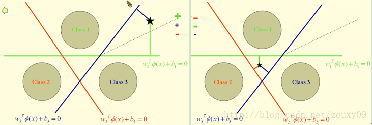
As shown below left. The red classification surface separates red from the other two colors, the green classification surface separates green from the other two colors, and the blue classification surface separates blue from the other two colors.
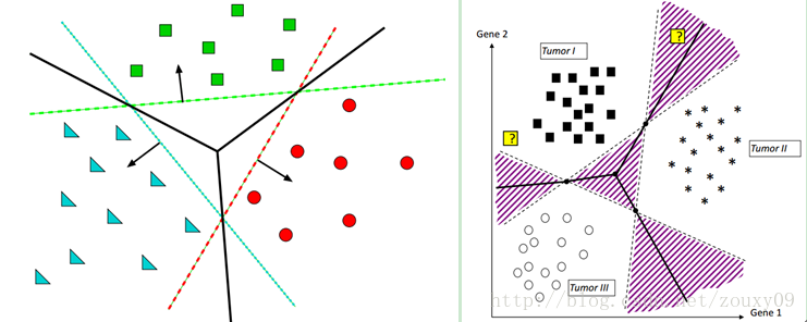
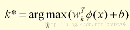
The classification of a point here is actually by measuring the distance from this point to the three decision boundaries, because the greater the distance to the classification surface, the more credible the classification is. Of course, this distance is signed as follows:
For example, the left of the figure below divides the point of stars into green. The picture on the right divides the point of stars into brown.
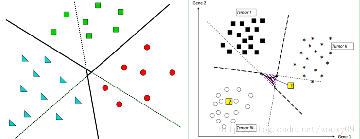
6.2. "One to one" method
The One-Against-One method is to select one class of samples at a time as the positive class sample, while the negative class sample is changed to only select one class (called a "one-on-one singled" method, oh no, there is no singled , Is the "one-on-one" method, huh), which avoids skew. Therefore, the process is to calculate such classifiers. The first one answers only "Is it the first or the second class?" The second one answers only "Is it the first or the third class?" Class or class 4 ", so if you continue, you can also immediately get that such a classifier should have 5 X 4/2 = 10 (the general formula is that if there are k classes, the total number of two classifiers K (k-1) / 2). Although the number of classifiers is larger, the total time used in the training phase (that is, when calculating the classification planes of these classifiers) is much less than the "one-class-to-the-other" method. The sample is thrown to all classifiers. The first classifier will vote to say that it is "1" or "2", and the second one will say that it is "1" or "3", and each will vote for it. , The final count of votes, if the category "1" received the most votes, it is judged that this article belongs to the first category. This method obviously also has the phenomenon of classification overlap, but there will be no non-classification, because it is always impossible to have 0 votes for all categories. As shown in the figure below, the purple block in the middle has 1 vote for each category, so you do n’t know which category to classify, you can only throw it to a certain category (or measure this point to three decision boundaries) Distance, because the larger the distance to the classification surface, the more credible the classification is). If you throw it away, you will be well off. If you throw it wrong, it will not be lucky.
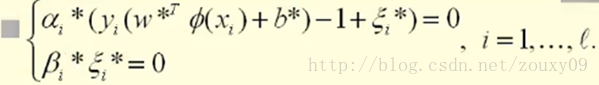
Analysis of KKT conditions
For KKT conditions, please refer to [13] [14]. Assume that the optimal solutions we get from optimization are: α i *, β i *, ξ i *, w *, and b * . Our optimal solution needs to satisfy the KKT condition:
At the same time, β i * and ξ i * both need to be greater than or equal to 0, and α i * needs to be between 0 and C. That can be discussed in three situations:
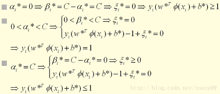
In general, the KKT condition becomes:
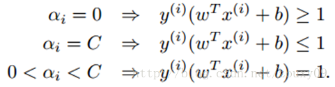
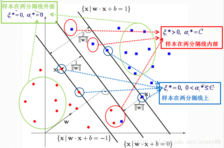
The first equation shows that if α i = 0, then the sample falls outside the two interval lines. The second formula shows that if α i = C, then the sample may fall inside or between two interval lines, depending on whether the value of the corresponding relaxation variable is equal to 0 or greater than 0. The third formula indicates that if 0 < α i <C, then the sample must fall on the dividing line (this is important, b is calculated by taking these points that fall on the dividing line, because on the dividing line w T x + b = 1 or -1 is the equation. In other places, it is an inequality, which cannot be solved by b). The specific visualization is as follows:
According to the KKT condition, it is known that α i that is not equal to 0 is a support vector, and it may fall on the separation line, or it may fall inside the two separation lines. The KKT condition is very important. In SMO, which is one of the implementation algorithms of SVM, we can see its important applications.
————————————————
版权声明:本文为CSDN博主「zouxy09」的原创文章,遵循 CC 4.0 BY-SA 版权协议,转载请附上原文出处链接及本声明。
原文链接:https://blog.csdn.net/zouxy09/article/details/17291805
মেশিন লার্নিং অ্যালগরিদম এবং পাইথন অনুশীলনের এই সিরিজটি মূলত "মেশিন লার্নিং ইন অ্যাকশন " বইয়ের উপর ভিত্তি করে তৈরি । যেহেতু আমি পাইথন শিখতে চাই এবং তারপরে আমি কিছু মেশিন লার্নিং অ্যালগরিদম সম্পর্কে আরও জানতে চাই, আমি পাইথনের মাধ্যমে আরও বেশ কয়েকটি ব্যবহৃত ব্যবহৃত মেশিন লার্নিং অ্যালগরিদম বাস্তবায়ন করতে চাই। আমি এই একইমুখী বইয়ের সাথে দেখা করতে পেরেছি, তাই আমি এই বইটির প্রক্রিয়াটি শিখতে ব্যবহার করেছি।
এই বিভাগে, আমরা মূলত এসভিএম সিস্টেমটি পর্যালোচনা করি এবং পাইথনের মাধ্যমে এটি প্রয়োগ করি। যেহেতু এখানে প্রচুর সামগ্রী রয়েছে তাই এখানে তিনটি ব্লগ পোস্ট রয়েছে। প্রথমটি এসভিএমের বেসিক সম্পর্কে, দ্বিতীয়টি অ্যাডভান্সডগুলি সম্পর্কে, যা মূলত এসভিএমের পুরো জ্ঞান চেইনটিকে সোজা করে এবং তৃতীয়টি পাইথনের বাস্তবায়ন প্রবর্তন করে। এসভিএমের খুব ভাল ব্লগ পোস্ট রয়েছে, আপনি এই নিবন্ধে তালিকাভুক্ত রেফারেন্সগুলি এবং প্রস্তাবিত পাঠগুলি উল্লেখ করতে পারেন। এই নিবন্ধে, অবস্থানটি হ'ল সংহত এসভিএমের সামগ্রিক জ্ঞান চেনাকে সোজা করা, যাতে এটি বিশদ অনুসন্ধানের সাথে জড়িত না। ইন্টারনেটে অনেক ভাল ছাড় এবং বই রয়েছে এবং আপনি সেগুলি উল্লেখ করতে পারেন।
নির্দেশিকা
I. ভূমিকা
দ্বিতীয়ত, রৈখিকভাবে পৃথকযোগ্য এসভিএম এবং হার্ড অন্তর সর্বাধিককরণ
তৃতীয়ত, দ্বৈত অপ্টিমাইজেশান সমস্যা
৩.১ দ্বৈততা
৩.২ এসভিএম অপটিমাইজেশনের দ্বৈত সমস্যা
চতুর্থত, শিথিলকরণ ভেক্টর এবং নরম বিরতি সর্বাধিককরণ
পাঁচ, কার্নেল ফাংশন
ছয়, বহু শ্রেণির শ্রেণিবিন্যাস এসভিএম
6.1, "এক থেকে বহু" পদ্ধতি
One.২। "এক থেকে এক" পদ্ধতি
কেকেটি অবস্থার বিশ্লেষণ
আট, এসএমও অ্যালগরিদমের এসএমও বাস্তবায়ন
8.1 সমন্বিত বংশদ্ভুত অ্যালগরিদম
8.2, এসএমও অ্যালগরিদম নীতি
৮.৩. এসএমও অ্যালগরিদমের পাইথন বাস্তবায়ন
রেফারেন্স এবং প্রস্তাবিত পড়া
পাঁচ, কার্নেল ফাংশন
যদি আমাদের সাধারণ নমুনা বিতরণটি নীচের চিত্রের বাম দিকে দেখানো হয়, তবে এটি স্বাভাবিক হওয়ার কারণটি বোঝায় যে উপরোক্ত কিছু জেদী বহিরাগতদের কারণে এটি রৈখিক অবিভাজ্য নয়। এটি সত্যই লিনিয়ার এবং অবিভাজ্য। নমুনার বিতরণ নিজেই এর মতো you আপনি যদি নমুনার মতো শিথিলকরণ ভেরিয়েবলের মাধ্যমে লিনিয়ার শ্রেণিবিন্যাসের সীমাটিও বাইরে বের করেন তবে স্পষ্টতই বোঝা যায় যে এই শ্রেণিবদ্ধকরণ পৃষ্ঠটি খুব খারাপ। আমাদের কী করা উচিত? রৈখিকভাবে পৃথকযোগ্য ডেটাগুলির জন্য এসভিএম কার্যকর se অবিচ্ছেদ্যতার জন্য কিছু ভাল কৌশল কী কী? কার্নেল ট্রিকের সময় এসেছে।
উপরের চিত্রের ডানদিকে যেমন প্রদর্শিত হয়েছে, আমরা যদি আমাদের মূল নমুনা পয়েন্টগুলিকে অন্য বৈশিষ্ট্য স্থানে রূপান্তর করতে পারি, যা এই বৈশিষ্ট্য স্পেসে রৈখিকভাবে পৃথকযোগ্য, তবে উপরের এসভিএম সহজেই কাজ করতে পারে। তা হল, অবিচ্ছেদ্য উপাত্তের জন্য আমাদের এখন দুটি জিনিস করা দরকার:
1) প্রথমে সমস্ত মূল ডেটা এক্সকে অন্য বৈশিষ্ট্যের জায়গাতে রূপান্তর করতে প্রথমে একটি অ-রৈখিক ম্যাপিং use ( x ) ব্যবহার করুন , যাতে নমুনাগুলি লৈখিকভাবে পৃথক হয়ে যায়;
2) তারপরে শ্রেণিবিন্যাস শেখার জন্য বৈশিষ্ট্য স্পেসে এসভিএম ব্যবহার করুন।
ঠিক আছে, আগের মতো দ্বিতীয় কাজ সম্পর্কে কিছু বলার নেই। কে প্রথম ভারী কাজ করবে? আমরা কীভাবে জানব যে কোন রূপান্তরটি আমাদের ডেটাগুলিকে রৈখিক বিচ্ছিন্ন হতে মানচিত্র করতে পারে? ডেটা মাত্রা এত বড় যে আমরা এটি দেখতে পারি না। তদ্ব্যতীত, এই রূপান্তরটি কি দ্বিতীয় পদক্ষেপের অপ্টিমাইজেশনকে জটিল করে তুলবে এবং আরও গণনামূলকভাবে ব্যয়বহুল করবে? প্রথম সমস্যার জন্য, একটি সুপরিচিত প্রচ্ছদ উপপাদ্য রয়েছে: একটি জটিল প্যাটার্ন শ্রেণিবিন্যাসের সমস্যাটি নিম্ন-মাত্রিক স্থানের তুলনায় অরেখরীয়ভাবে নিম্ন-মাত্রিক স্থানের তুলনায় লিনিয়ারে পৃথক হওয়ার সম্ভাবনা বেশি। ঠিক আছে, এটি সহজ, আমাদের একটি ম্যাপিং সন্ধান করতে হবে যেখানে সমস্ত নমুনা উচ্চতর মাত্রিক স্থানে ম্যাপ করা হয়। দুঃখিত, এই ম্যাপিং ফাংশনটি খুঁজে পাওয়া আসলে খুব কঠিন। যাইহোক, সমর্থন ভেক্টর মেশিন সরাসরি এই জটিল অ-রৈখিক রূপান্তর সনাক্ত এবং গণনা করে না, বরং বুদ্ধিমানভাবে একটি চৌকস সার্কিটাস পদ্ধতির মাধ্যমে পরোক্ষভাবে এই রূপান্তরটি প্রয়োগ করে। এটি কার্নেল ফাংশন, যার মধ্যে কেবল এই সুপার পাওয়ার নেই, তবে উভয় বিশ্বের সেরাের গণনা ব্যয়ও বাড়ায় না। আমরা উপরের এসভিএমের অপ্টিমাইজেশান সমস্যার দিকে ফিরে তাকাতে পারি:
এটি দেখা যায় যে নমুনা এক্স ব্যবহারের জন্য , কেবলমাত্র আই-তম এবং জে-তম নমুনার অভ্যন্তরীণ পণ্য গণনা করা প্রয়োজন।
শ্রেণিবদ্ধকরণ সিদ্ধান্তের কার্যের জন্য, দুটি নমুনার অভ্যন্তরীণ পণ্যও গণনা করা হয়। এটি, এসভিএম প্রশিক্ষণ এবং এসভিএম ব্যবহার উভয়ই নমুনার মধ্যে অভ্যন্তরীণ পণ্য ব্যবহার করে এবং কেবল অভ্যন্তরীণ পণ্য ব্যবহার করা হয়। তারপরে যদি আমরা একটি উচ্চ মাত্রিক স্থানটিতে ম্যাপযুক্ত দুটি নমুনার অভ্যন্তরীণ মানের মূল্য গণনা করার উপায় খুঁজে পাই। কার্নেল ফাংশনটি এই দুর্দান্ত মিশনটি সম্পাদন করে:
কে ( এক্স আই , এক্স জে ) = Φ ( এক্স আই ) টি Φ ( এক্স জে )
অর্থাত দুটি নমুনা এক্স আমি এবং এক্স জে অভ্যন্তরীণ পণ্য সংশ্লিষ্ট [Phi] একটি উচ্চ মাত্রিক স্থান ( এক্স আমি ) টি [Phi] ( এক্স জে ) একটি কার্নেল ফাংশন কে মাধ্যমে ( এক্স আমি , এক্স জে হিসাব)। কে এই রূপান্তর knowing ( এক্স ) তা না জেনে । এবং এই কার্নেল ফাংশনের গণনা খুব সহজ The রেডিয়াল ভিত্তি আরবিএফ ফাংশনটি সাধারণত ব্যবহৃত হয়:
এই মুহুর্তে, আমাদের অনুকূলিত দ্বৈত সমস্যাটি হয়ে ওঠে:
পূর্ববর্তী অপ্টিমাইজেশান সমস্যা থেকে একমাত্র পার্থক্য হ'ল নমুনাগুলির অভ্যন্তরীণ পণ্যটি কার্নেল ফাংশন দিয়ে প্রতিস্থাপন করা দরকার। অপ্টিমাইজেশন প্রক্রিয়াটিতে কোনও পার্থক্য নেই। এবং সিদ্ধান্তের কার্যটি হয়ে যায়:
এটি হ'ল নতুন নমুনা এক্স এবং আমাদের সমস্ত প্রশিক্ষণের নমুনাগুলি কার্নেল ফাংশন গণনা করতে ব্যবহার করা যেতে পারে। এটি লক্ষ করা উচিত যে কারণ বেশিরভাগ নমুনার মধ্যে ল্যাংরেজ ফ্যাক্টর α i , আসলে, আমাদের কেবলমাত্র কয়েকটি সংখ্যক প্রশিক্ষণের নমুনা এবং নতুন নমুনাগুলির কার্নেল ফাংশনটি গণনা করতে হবে, এবং তারপরে যোগ করতে হবে এবং নতুনটি সম্পূর্ণ করতে সাইনটি গ্রহণ করতে হবে এখানে নমুনা x এর শ্রেণিবিন্যাস আসে । সমর্থন ভেক্টর মেশিনের সিদ্ধান্ত প্রক্রিয়াটিকেও একটি মিলের তুলনা প্রক্রিয়া হিসাবে বিবেচনা করা যেতে পারে। প্রথমত, ইনপুট নমুনাগুলি একাধিক টেম্পলেট নমুনাগুলির সাথে তুলনা করা হয় The টেম্পলেট নমুনাগুলি প্রশিক্ষণ প্রক্রিয়া দ্বারা নির্ধারিত সমর্থন ভেক্টর এবং ব্যবহৃত সদৃশতাটি কর্নেল ফাংশন। সমর্থন ভেক্টর ভরযুক্ত সমষ্টি পর প্রতিটি নমুনা স্কোর তুলনা করার পর, ওজন সহগ প্রতিটি SVM প্রশিক্ষণের জন্য প্রাপ্ত হয় [আলফা] আমি এবং বিভাগ লেবেল ফলাফল নেই। অবশেষে, ওজনফলের পরিমাণের ভিত্তিতে সিদ্ধান্ত নেওয়া হয়। এবং বিভিন্ন কার্নেল ফাংশনগুলি ব্যবহার করে বিভিন্নতা মিলানোর বিভিন্ন পদ্ধতি ব্যবহারের সমতুল্য।
একটি গণনামূলক দৃষ্টিকোণ থেকে, Φ ( x ) রূপান্তরটির স্থানিক মাত্রা যত বেশি হোক না কেন , এমনকি একটি অসীম মাত্রা (ফাংশন অসীম মাত্রা), এই স্থানটিতে লিনিয়ার সাপোর্ট ভেক্টর মেশিনের সমাধানটি মূল স্থানটিতে কার্নেল ফাংশন দ্বারা সম্পাদন করা যেতে পারে। উচ্চ-মাত্রিক স্থানটিতে গণনা এড়ানো যায়, এবং কার্নেল ফাংশন গণনা করার জটিলতা এবং মূল নমুনার অভ্যন্তরীণ পণ্য গণনা করার জটিলতা যথেষ্ট পরিমাণে বৃদ্ধি পায় না।
এখানে, আমি দীর্ঘশ্বাস ফেললেও সাহায্য করতে পারি না। "ভেক্টর" এসভিএমকে কেন সর্বদা অভ্যন্তরীণ পণ্য আকারে গণনা করা দরকার? "কাকতালীয়ভাবে" কেন একটি কার্নেল ফাংশন বিদ্যমান রয়েছে যা ম্যাপিং স্পেসের অভ্যন্তরীণ পণ্য ক্রিয়াকে সহজতর করে? কেন সীমাবদ্ধতার মধ্যে সবচেয়ে বেশি নমুনাগুলি সিদ্ধান্তের সীমানায় শূন্য অবদান রাখে? … Thankশ্বরের ধন্যবাদ, বা বিশাল এবং মহান গবেষককে ধন্যবাদ! আমাকে এবং অন্যান্য সাধারণ মানুষ গণিতের এমন অপূর্ব এবং অতুলনীয় সৌন্দর্যের এক ঝলক দেখতে দিন!
এই মুহুর্তে, আমরা ভেক্টর মেশিনগুলি সমর্থন সম্পর্কিত জিনিসগুলি আবরণ করেছি। সংক্ষিপ্তসার হিসাবে: সমর্থন ভেক্টর মেশিনগুলির প্রাথমিক ধারণাটি সংক্ষেপে এইভাবে সংক্ষিপ্ত করা যায়: প্রথমে ইনপুট স্পেসটিকে অ-রৈখিক রূপান্তর মাধ্যমে একটি উচ্চ-মাত্রিক স্থানে রূপান্তর করুন এবং তারপরে অনুকূল শ্রেণিবদ্ধকরণ পৃষ্ঠটি আবিষ্কার করুন, এই নতুন স্থানটিতে সর্বাধিক ব্যবধান শ্রেণিবিন্যাস এবং এই অ- লিনিয়ার রূপান্তর একটি উপযুক্ত অভ্যন্তরীণ পণ্য কার্নেল ফাংশন সংজ্ঞায়িত করে অর্জিত হয়। কাঠামোগত ঝুঁকি হ্রাস করার নীতি অনুসারে স্ট্যাটিস্টিকাল লার্নিং তত্ত্ব অনুসারে এসভিএম আসলে প্রস্তাবিত হয় এটির দুটি লক্ষ্য প্রয়োজন: ১) দুই ধরণের সমস্যা পৃথক করা যায় (অভিজ্ঞতাগত ঝুঁকি হ্রাস করা হয়) 2) সর্বাধিক মার্জিন (সর্বনিম্ন ঝুঁকি উপরের আবদ্ধ) গ্যারান্টিযুক্ত কমপক্ষে অভিজ্ঞতামূলক ঝুঁকিযুক্ত ফাংশনটি সর্বনিম্ন ঝুঁকির সাথে সাবসেটে নির্বাচিত হয়।
ছয়, বহু শ্রেণির শ্রেণিবিন্যাস এসভিএম
এসভিএম হ'ল একটি সাধারণ দ্বি-শ্রেণীর শ্রেণিবদ্ধকারী, এটি কেবল ইতিবাচক বা নেতিবাচক শ্রেণীর অন্তর্ভুক্ত কিনা এই প্রশ্নের উত্তর দেয়। বাস্তবে সমাধান হওয়া সমস্যাগুলি প্রায়শই একাধিক ধরণের সমস্যা problems সুতরাং আপনি কীভাবে একটি দ্বি-শ্রেণীর শ্রেণিবদ্ধের কাছ থেকে একটি বহু-শ্রেণীর শ্রেণিবদ্ধী পাবেন?
6.1, "এক থেকে বহু" পদ্ধতি
ওয়ান-অ্যাসিস্ট-অল এখনও ভাবা অপেক্ষাকৃত সহজ। প্রতিবার দ্বি-শ্রেণীর শ্রেণিবিন্যাসের সমস্যাটি সমাধান করা। উদাহরণস্বরূপ, আমাদের 5 টি বিভাগ রয়েছে the প্রথমবারের জন্য, বিভাগ 1 এর নমুনাগুলি ধনাত্মক নমুনা হিসাবে নির্ধারিত হয়, এবং অবশিষ্ট 2, 3, 4, এবং 5 টি নমুনা negativeণাত্মক নমুনা হিসাবে মিলিত হয় this এইভাবে একটি দ্বি-শ্রেণির শ্রেণিবদ্ধ প্রাপ্ত হয়, যা একটি নমুনা নির্দেশ করতে পারে। এটি কি এখনও ক্লাস 1; দ্বিতীয়বার আমরা 2 বিভাগের নমুনাগুলিকে ধনাত্মক নমুনা হিসাবে সেট করেছিলাম এবং 1, 3, 4, 5 এর নমুনাগুলিকে এক শ্রেণিবদ্ধের জন্য নেতিবাচক নমুনা হিসাবে একত্রিত করেছি, এবং আরও, আমরা পেতে পারি এই জাতীয় 5 টি শ্রেণির শ্রেণিবদ্ধ (সর্বদা শ্রেণীর সংখ্যার সাথে সামঞ্জস্যপূর্ণ)। যখন কোনও নমুনাকে শ্রেণিবদ্ধ করার দরকার হয়, আমরা এই নমুনাটি নিই এবং প্রতিটি শ্রেণিবদ্ধকে একে একে জিজ্ঞাসা করি: এটি কি আপনার? এটা কি তোমার? কোন শ্রেণিবদ্ধক হু হু করে হ্যাঁ বলেছেন, নিবন্ধের বিভাগটি নির্ধারিত হয়েছিল। এই পদ্ধতির সুবিধাটি হ'ল প্রতিটি অপ্টিমাইজেশান সমস্যার আকার তুলনামূলকভাবে কম এবং শ্রেণিবিন্যাস দ্রুত হয় (ফলাফলগুলি জানতে এটি কেবল 5 শ্রেণিবদ্ধকারীদের কল করতে হবে)। তবে কখনও কখনও দুটি দুটি বিব্রতকর পরিস্থিতি যেমন: নমুনাকে একটি বৃত্ত জিজ্ঞাসা করার মতো, প্রতিটি শ্রেণিবদ্ধকারী বলে যে এটি তার শ্রেণীর অন্তর্গত, বা প্রতিটি শ্রেণিবদ্ধ ব্যক্তি বলে যে এটি তার শ্রেণি নয় পূর্ববর্তীটিকে শ্রেণিবিন্যাস ওভারল্যাপ প্রপঞ্চ বলা হয়, এবং পরবর্তীটিকে অস্বস্তিকর ঘটনা বলে। শ্রেণিবদ্ধকরণ ওভারল্যাপগুলি হ্যান্ডেল করা সহজ any কোনও একটি ফলাফল চয়ন করা বা এই নিবন্ধ থেকে প্রতিটি হাইপারপ্লেনের দূরত্বটি দেখুন, যে কোনওরকমই যাচাই করা খুব বিরক্তিজনক নয়। অবিশ্বাস্য ঘটনাটি সত্যিই কঠিন, এবং এটি কেবলমাত্র ষষ্ঠ বিভাগে বরাদ্দ করা যেতে পারে ... আরও ভয়ঙ্করভাবে, প্রতিটি বিভাগে নমুনার সংখ্যা প্রায় একই, তবে "অবশিষ্ট" বিভাগে নমুনার সংখ্যা সর্বদা ধনাত্মক শ্রেণীর চেয়ে বেশ কয়েকগুণ বেশি (কারণ এটি ইতিবাচক শ্রেণি ব্যতীত অন্যান্য শ্রেণি থেকে প্রাপ্ত নমুনাগুলির যোগফল), যা কৃত্রিমভাবে পূর্ববর্তী বিভাগে উল্লিখিত "ডেটা সেট স্কিউ" সমস্যা তৈরি করেছিল।
বাম নীচে প্রদর্শিত হিসাবে। লাল শ্রেণিবদ্ধকরণ পৃষ্ঠটি দুটি দুটি বর্ণ থেকে লালকে পৃথক করে, সবুজ শ্রেণিবদ্ধকরণ পৃষ্ঠটি দুটি দুটি বর্ণের থেকে সবুজকে পৃথক করে এবং নীল শ্রেণিবদ্ধকরণ পৃষ্ঠটি দুটি দুটি বর্ণের থেকে নীলকে পৃথক করে।
এখানে একটি বিন্দুর শ্রেণিবদ্ধকরণ আসলে এই বিন্দু থেকে তিনটি সিদ্ধান্তের সীমানার দূরত্ব পরিমাপের মাধ্যমে, কারণ শ্রেণিবিন্যাসের পৃষ্ঠের যত বেশি দূরত্ব হয়, শ্রেণিবিন্যাস তত বেশি বিশ্বাসযোগ্য। অবশ্যই, এই দূরত্বটি নিম্নরূপে স্বাক্ষরিত হয়েছে:
উদাহরণস্বরূপ, নীচের চিত্রের বাম তারার বিন্দুকে সবুজ করে ides ডান দিকের ছবিটি তারাগুলির বিন্দুকে বাদামি করে।
One.২। "এক থেকে এক" পদ্ধতি
ওয়ান-অ্যানজিস্ট-ওয়ান পদ্ধতিটি হ'ল ধনাত্মক শ্রেণির নমুনা হিসাবে একবারে একটি শ্রেণির নমুনা নির্বাচন করা হয়, যখন নেতিবাচক শ্রেণির নমুনাটি কেবলমাত্র একটি শ্রেণি নির্বাচন করা হয় (একে "এক-ও-ওয়ান সিঙ্গলড আউট" পদ্ধতি বলা হয়, ওহ, কোনও একক আউট নেই) , হ'ল "ওয়ান-ওয়ান" পদ্ধতি, হু) যা স্কু এড়িয়ে চলে। সুতরাং, প্রক্রিয়াটি এই জাতীয় শ্রেণিবদ্ধকারী গণনা করা হয় The প্রথমটির উত্তর কেবলমাত্র "এটি প্রথম বা দ্বিতীয় শ্রেণি?" দ্বিতীয়টি কেবল উত্তর দেয় "এটি কি প্রথম বা তৃতীয় শ্রেণি?" ক্লাস বা ক্লাস 4 ", সুতরাং আপনি অবিরত থাকলে আপনি অবিলম্বে এটি পেতে পারেন যে এই ধরণের শ্রেণিবদ্ধের 5 টি 4 4/2 = 10 হওয়া উচিত (সাধারণ সূত্রটি হল যদি কে ক্লাস থাকে তবে মোট দুটি শ্রেণিবদ্ধের সংখ্যা) কে (কে -১) / ২)। শ্রেণিবদ্ধের সংখ্যা বৃহত্তর হলেও, প্রশিক্ষণ পর্বে ব্যবহৃত মোট সময় (অর্থাত্ এই শ্রেণিবদ্ধের শ্রেণিবিন্যাসের বিমানগুলি গণনা করার সময়) "এক-শ্রেণীর থেকে অন্য" পদ্ধতির চেয়ে অনেক কম। নমুনাটি সমস্ত শ্রেণিবদ্ধের জন্য নিক্ষেপ করা হয় The প্রথম শ্রেণিবদ্ধ এটি "1" বা "2" বলে ভোট দেবে এবং দ্বিতীয়জন বলবে এটি "1" বা "3", এবং প্রত্যেকে এটির পক্ষে ভোট দেবে। , ভোটের চূড়ান্ত গণনা, "1" বিভাগে সর্বাধিক ভোট প্রাপ্ত হলে বিচার করা হয় যে এই নিবন্ধটি প্রথম বিভাগের অন্তর্গত। এই পদ্ধতির স্পষ্টতই শ্রেণিবিন্যাসের ওভারল্যাপের ঘটনাটিও রয়েছে, তবে কোনও শ্রেণিবিন্যাস থাকবে না, কারণ সব বিভাগের জন্য 0 ভোট পাওয়া সর্বদা অসম্ভব। নীচের চিত্রটিতে যেমন দেখানো হয়েছে, মাঝখানের বেগুনি ব্লকটিতে প্রতিটি বিভাগের জন্য 1 টি ভোট রয়েছে, তাই আপনি জানেন না কোন বিভাগটি শ্রেণিবদ্ধ করতে হবে, আপনি কেবলমাত্র এটি একটি নির্দিষ্ট বিভাগে ফেলে দিতে পারেন (বা এই বিষয়টিকে তিনটি সিদ্ধান্তের সীমানায় পরিমাপ করুন) দূরত্ব, কারণ শ্রেণিবিন্যাসের পৃষ্ঠের বেশি দূরত্ব, শ্রেণিবিন্যাস আরও বিশ্বাসযোগ্য) you আপনি যদি এটিকে ফেলে দেন তবে আপনি ভাল থাকবেন you যদি আপনি এটি ভুলভাবে ফেলে দেন তবে এটি ভাগ্যবান হবে না।
কেকেটি অবস্থার বিশ্লেষণ
কে কেটি অবস্থার জন্য, দয়া করে [13] [14] দেখুন। ধরে নিই যে অপটিমাইজেশন থেকে আমরা পাই সর্বোত্তম সমাধানগুলি হ'ল : α i *, β i *, ξ i *, w *, এবং b * । আমাদের অনুকূল সমাধানটির জন্য কেকেটি শর্তটি পূরণ করতে হবে:
একই সাথে, β i * এবং ξ i * উভয়ই 0 এর চেয়ে বড় বা সমান হতে হবে এবং α i * 0 এবং C এর মধ্যে হওয়া দরকার needs এটি তিনটি পরিস্থিতিতে আলোচনা করা যেতে পারে:
সাধারণভাবে, কেকেটি শর্তটি হয়ে যায়:
প্রথম সমীকরণটি দেখায় যে যদি α i = 0 হয় তবে নমুনাটি দুটি বিরতিরেখার বাইরে চলে যায়। দ্বিতীয় সূত্রটি দেখায় যে যদি α i = C হয় তবে সংশ্লিষ্ট শিথিলকরণের ভেরিয়েবলের মান 0 বা তার চেয়ে বড় হবে কিনা তার উপর নির্ভর করে নমুনাটি দুটি অন্তরাল লাইনের অভ্যন্তরে বা দুটি ব্যবধানের মধ্যে পড়তে পারে। তৃতীয় সূত্রটি সূচিত করে যে যদি 0 < α i <C হয়, তবে নমুনাটি অবশ্যই বিভাজনরেখার উপর পড়তে হবে (এটি গুরুত্বপূর্ণ, বি বিভাজনরেখার উপর পড়ে এই পয়েন্টগুলি গ্রহণ করে গণনা করা হয়, কারণ ডাব্লু টি এক্স + বি = 1 বা -1 সমীকরণ। অন্যান্য জায়গায় এটি একটি অসমতা, যা খ দ্বারা সমাধান করা যায় না)। নির্দিষ্ট দৃশ্যায়নটি নিম্নরূপ:
Kkt অবস্থা, বোঝা [আলফা] আমি 0 ভেক্টর সমান নয় সমর্থিত, এটা বিভাজক লাইনে পড়তে পারে, এছাড়াও দুটি পৃথক লাইন ভিতরে পড়া হতে পারে। কেকেটি শর্তটি অত্যন্ত গুরুত্বপূর্ণ SM এসএমএম-এ, যা এসভিএম এর বাস্তবায়ন অ্যালগরিদমগুলির মধ্যে একটি, আমরা এর গুরুত্বপূর্ণ প্রয়োগগুলি দেখতে পাই।
————————————————
版权声明:本文为CSDN博主「zouxy09」的原创文章,遵循 CC 4.0 BY-SA 版权协议,转载请附上原文出处链接及本声明。
原文链接:https://blog.csdn.net/zouxy09/article/details/17291805
0 comments:
Post a Comment