This series of machine learning algorithms and Python practice is mainly based on the book "Machine Learning in Action " . Because I want to learn Python, and then I want to learn more about some machine learning algorithms, I want to implement several more commonly used machine learning algorithms through Python. I happened to meet this samely-oriented book, so I used the process of this book to learn.

       In this section, we mainly review the SVM system and implement it through Python. Since there is so much content, here are three blog posts. The first one is about the basics of SVM, the second is about the advanced ones, which mainly straightens the entire knowledge chain of SVM, and the third one introduces the implementation of Python. SVM has a lot of very good blog posts, you can refer to the references and recommended readings listed in this article. In this article, the positioning is to straighten out the overall knowledge chain of the integrated SVM, so it will not involve the derivation of details. There are many good deductions and books on the Internet, and you can refer to them.

table of Contents

I. Introduction

Second, linearly separable SVM and hard interval maximization

Third, the dual optimization problem

       3.1 Duality

       3.2 Dual Problem of SVM Optimization

Fourth, relaxation vector and soft interval maximization

Five, the kernel function

Six, multi-class classification SVM

       6.1, "One-to-many" method

       6.2. "One to one" method

Analysis of KKT conditions

Eight, SMO implementation of SMO algorithm

       8.1 Coordinate descent algorithm

       8.2, SMO algorithm principle

       8.3.Python implementation of SMO algorithm

References and recommended reading

Eight, SMO implementation of SMO algorithm

      Finally to the implementation part of SVM. Then the magical and effective things have to return to realization before they can show their powerful skills. SVM is effective and there are very efficient training algorithms, which is why SVM is very popular in industry.

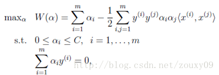
      As mentioned earlier, the learning problem of SVM can be transformed into the following dual problem:

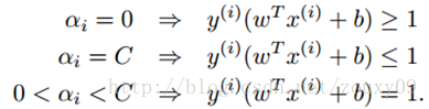
       KKT conditions to be met:

       In other words, finding a set of α i that can meet the above conditions is an optimal solution for the goal. So our optimization goal is to find the optimal set of α i *. Once these α i * are obtained , it is easy to calculate the weight vectors w * and b and get the separated hyperplane.

       This is a convex quadratic programming problem, which has a global optimal solution, which can generally be optimized by existing tools. However, when there are many training samples, these optimization algorithms are often time-consuming and inefficient, making them unusable. From SVM to the present, many methods for optimizing training have also appeared. Among them, the most famous one is the Sequential Minimal Optimization sequence minimization optimization algorithm, referred to as the SMO algorithm, proposed by John C. Platt of Microsoft Research in the paper "Sequential Minimal Optimization: A Fast Algorithm for Training Support Vector Machines" in 1982. The idea of ​​the SMO algorithm is very simple, it decomposes a large optimization problem into multiple small optimization problems. These small problems are often easier to solve, and the results of sequentially solving them are completely consistent with the results of solving them as a whole. While the results are completely consistent, the solution time of SMO is much shorter. Before diving into the SMO algorithm, let's first understand the algorithm of coordinate descent. SMO is actually based on this simple idea.

8.1 Coordinate descent (rise) method

      Suppose the following optimization problem is required:

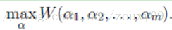
      Here, we need to solve m variables α i , generally through gradient descent (here is to find the maximum value, so it should be called ascending) and other algorithms for each iteration of all m variables α i that is the α vector optimization. The value of each element in the alpha vector is adjusted by each iteration through the error . The coordinate rise method (coordinate rise and coordinate fall can be regarded as a pair, the coordinate rise is used to solve the max optimization problem, and the coordinate fall is used to find the min optimization problem). The idea is to adjust only one variable α i per iteration. The values ​​of other variables are fixed in this iteration.

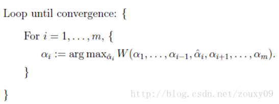
       The meaning of the innermost sentence is to fix all α j except α i (i is not equal to j). At this time, W can be regarded as only a function about α i , then the derivative of α i can be optimized directly . Here, the order i for maximizing differentiation is from 1 to m. We can change the optimization order to make W increase and converge faster. If W can reach the optimum quickly in the inner loop, then the coordinate rising method will be a very efficient method of finding the extreme value.

      A two-dimensional example is used to illustrate the coordinate descent method: we need to find (x *, y *) at the minimum value of f (x, y) = x 2 + xy + y 2 , which is also F * in the figure below Point somewhere.

       Suppose our initial point is A (the figure is a contour map of the function projected onto the xoy plane, the darker the value, the smaller the value). We need to reach the point where F *. The fastest method is the path of the yellow line in the figure, which arrives at one time. In fact, this is Newton's optimization method, but if it is high-dimensional, this method is not very efficient (because the inverse of the matrix needs to be solved, this is not Discussed here). We can also follow the path indicated in red. Starting from A, first fix x, walk along the y-axis to the point where f (x, y) decreases, and then fix y, and then follow the x-axis to decrease the value of f (x, y). Go to point C and continue to cycle until you reach F *. Anyway, as long as we go to the place where the value of f (x, y) is small, so that we can walk down step by step, each step will make f (x, y) gradually smaller. One day, the emperor will not Caring. Reaching F * is also a matter of time. At this point, you might say that the gap between the rich and the poor on the red line is too serious. Because here is a two-dimensional simple case. If it is a high-dimensional situation, and the objective function is complicated, plus a large number of sample sets, then in gradient descent, the objective function finds the gradient of all α i or inverts the matrix in Newton's method, which is very time-consuming. of. At this time, if W only optimizes a single α i quickly, the coordinate descent method may be more efficient.

8.2 SMO algorithm

       The idea of ​​the SMO algorithm is similar to that of the coordinate descent method. The only difference is that SMO is an iterative optimization of two α instead of one. Why optimize both?

       We return to this optimization problem. We can see that there is a constraint in this optimization problem, that is,

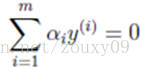
       Suppose we first fix all parameters except α 1 and then find the extreme value on α 1 . However, it should be noted that if all parameters other than α 1 are fixed , it can be known from the above constraint that α 1 will no longer be a variable (which can be deduced from other values), because the question specifies:

      Therefore, we need to select two parameters at a time for optimization, such as α i and α j . At this time, α i can be expressed by α j and other parameters. Substituting W in this way, W is only a function of α j . At this time, only α j can be optimized. Here is the derivation of α j . Let the derivative be 0 to solve the optimal α j at this time . Α i can then also be obtained . This is an iterative process. One iteration only adjusts the two Lagrangian multipliers α i and α j . SMO is efficient because after fixing other parameters, the optimization process for one parameter is very efficient (the optimization of a parameter can be solved analytically, not iteratively. Although a minimum optimization of a parameter cannot guarantee that the result is optimized The final result of the Lagrangian multiplier, but will make the objective function go to a minimum, so that all the multipliers are minimized until the objective function reaches the minimum when all the KKT conditions are met).

       To sum it up:

Repeat the process until convergence {

(1) Select two Lagrangian multipliers α i and α j ;

(2) Fix other Lagrange multipliers α k (k is not equal to i and j), and optimize w ( α ) only for α i and α j ;

(3) Update the value of the intercept b according to the optimized α i and α j ;

}

        So how are these two or three steps implemented in training, and what needs to be considered? Let's analyze it in detail:

(1) Select α i and α j :

        We are now optimizing the two Lagrange multipliers α i and α j of the objective function with each iteration , and then the other Lagrangian multipliers remain fixed. If there are N training samples, we have N Lagrangian multipliers that need to be optimized, but each time we pick only two for optimization, we have N (N-1) choices. So which pair of α i and α j do we choose ? Which one is better? Think about our goals? We hope to correct all the samples that violate the KKT conditions, because if all the samples meet the KKT conditions, our optimization is complete. That's very intuitive. Which black horse is the most serious, we have to educate him first to get him back to the right path as soon as possible. OK, then the first variable α i we choose is the one that violates the most severe KKT conditions. How to choose the second variable α j ?

       We want to find the optimal N Lagrangian multipliers quickly so that the cost function is maximized. In other words, we need to find the N Lagrangian multipliers corresponding to the place where the maximum value of the cost function is the fastest. This way our training time will be short. Just like when you go from Guangzhou to Beijing, there are planes and green cars for you to choose. What do you choose? (Even if you don't think about speed, you have to think about the feelings of the stewardess, don't live up to their expectations of seeing you, haha). A bit off topic, anyway, in each iteration, which pair of α i and α j can let me reach the place where the cost function value is the largest, we choose them. In other words, after this step, the value of the cost function of this pair of α i and α j is selected to increase the most, which is more than that of all other combinations of α i and α j . In this way, we can approach the maximum value of the cost function faster, which is to reach the goal of optimization. For another example, in the figure below, we need to walk from point A to point B. When we follow the blue route and go in the direction of c2, we take a big step. step. Therefore, the blue route takes two steps to enter the door of success, while the red route has twists and turns of life, as if success is far away, so choice is more important than hard work!

       Really! After talking for a long time, in fact, there is only one sentence: why the best α i and α j should be selected for each iteration , just to achieve faster convergence! So how to choose α i and α j for each iteration in practice ? This has a nice name called heuristic selection. The main idea is to first select the α i that is most likely to need optimization (that is, the violation of the KKT condition is the most serious) , and then choose the α i that is most likely to obtain a larger correction step. Long α j . Specifically, the following two processes:

1) Selection of the first variable α i :

       SMO calls the process of selecting the first variable the outer loop. Outer training selects the sample points with the worst KKT conditions in the training samples. And use its corresponding variable as the first variable. Specifically, test whether the training samples (x i , y i ) meet the KKT condition, that is:

       The test is performed in the ε range. In the inspection process, the outer loop first traverses all the sample points that satisfy the condition 0 <α j <C, that is, the support vector points on the interval boundary, checks whether they meet the KKT condition, and then selects the α i that violates the KKT condition most seriously . If these sample points all meet the KKT condition, then traverse the entire training set, check whether they meet the KKT condition, and then select the α i that violates the KKT condition most seriously .

       It is preferred to traverse non-boundary data samples, because non-boundary data samples are more likely to need adjustment, and boundary data samples often cannot be further adjusted and remain on the boundary. Since most of the data samples are obviously impossible to be support vectors, once the corresponding α multiplier obtains a zero value, there is no need to adjust it. Iterate through the non-boundary data samples and select the ones that violate the KKT condition. When a traversal finds that no non-boundary data samples have been adjusted, all data samples are traversed to check whether the entire set meets the KKT condition. If data samples are further evolved in the test of the entire set, it is necessary to traverse the non-boundary data samples. In this way, it constantly switches between traversing all data samples and traversing non-boundary data samples until the entire sample set meets the KKT condition. The above tests on the data samples using the KKT condition are all based on the condition that it can be stopped with a certain accuracy ε. If very accurate output algorithms are required, they often fail to converge quickly.

       The traversal scan of the entire data set is quite easy. When implementing the scan of non-boundary α i , the α i value of all non-boundary samples (that is, 0 <α i <C) must be saved to a new list. And then iterate through them. At the same time, this step skips those known α i values that will not change .

2) Selection of the second variable α j :

       After selecting the first α i , the algorithm selects the second α j value through an inner loop . Because the iterative step size of the second multiplier is roughly proportional to | E i -E j |, we need to choose the second multiplier that maximizes | E i -E j | Two multipliers). Here, in order to save calculation time, we set up a global cache to store the error values ​​of all samples, instead of recalculating each time it is selected. We choose α j which maximizes the step size or | E i -E j | max .

(2) Optimize α i and α j :

       After selecting these two Lagrangian multipliers, we need to first calculate the constraint values ​​for these parameters. Then solve this constraint maximization problem.

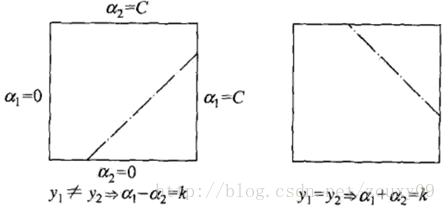
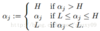
       First, we need to give [alpha] J find the boundary L <= [alpha] J <= H, to ensure that the [alpha] J satisfying 0 <[alpha] = J <= C of constraints. This means that α j must fall into this box. Since there are only two variables (α i , α j ), the constraint can be represented by a graph in a two-dimensional space, as shown below:

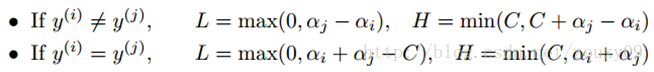
       The inequality constraint makes (α i , α j ) inside the box [0, C] x [0, C], and the equality constraint makes (α i , α j ) parallel to the box [0, C] x [0, C ] On a straight straight line. So what is required is the optimal value of the objective function on a line segment parallel to the diagonal. This makes the two-variable optimization problem a substantial one-variable optimization problem. From the figure, the upper and lower bounds of α j can be obtained by the following method:

       When we optimize, α j must satisfy the above constraint. In other words, the above is the feasible region of α j . Then we start looking for α j to maximize the objective function. The updated formula for α j obtained by derivation is as follows:

       Here E k can be regarded as the k-th sample, the output of the SVM and the expected output, that is, the error of the sample label.

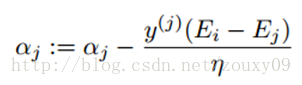
       And η actually measures the similarity of the two samples i and j. When calculating η, we need to use the kernel function, so we can use the kernel function to replace the inner product above.

       After obtaining the new α j , we need to ensure that it is within the boundary. In other words, if this optimized value ran out of the boundaries L and H, we need to simply crop and bring α j back into this range:

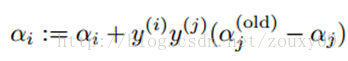
       Finally, after getting the optimized α j , we need to use it to calculate α i :

       At this point, the optimization of α i and α j is complete.

(3) Calculate the threshold b:

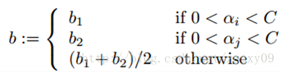
       After optimizing α i and α j , we can update the threshold b so that the KKT condition is satisfied for both samples i and j. If α i is not on the boundary after optimization (that is, satisfies 0 <α i <C, then according to the KKT condition, we can get y i g i (x i ) = 1, so we can calculate b), then the following threshold value b1 is valid because it forces the SVM to output y i when x i is input .

       Similarly, if 0 <α j <C, then the following b2 is also valid:

      If 0 <α i <C and 0 <α j <C are satisfied, then b1 and b2 are both valid, and they are equal. If both of them are on the boundary (that is, α i = 0 or α i = C, and α j = 0 or α j = C), then the threshold between b1 and b2 meets the KKT condition. Generally, we take Their average is b = (b1 + b2) / 2. So, in general, the update to b is as follows:

       Every time the minimum optimization is done, the error of each data sample must be updated in order to face the other data samples with the modified classification, and then used to estimate the step size when selecting the second paired optimized data sample.

(4) Termination conditions for convex optimization problems:

       The basic idea of ​​the SMO algorithm is: If the solutions with variables all satisfy the KKT condition of this optimization problem, then the solution of this optimization problem is obtained. Because the KKT condition is a necessary and sufficient condition for the optimization problem (please refer to the reference for proof). So we can monitor the KKT condition of the original problem, so all the samples meet the KKT condition, then the iteration is over. However, since the KKT condition itself is relatively harsh, it is also necessary to set a tolerance value, that is, if all the samples meet the KKT condition within the tolerance value range, the training can be concluded; of course, there are other termination conditions for the convex optimization of the dual problem You can refer to the literature.

8.3.Python implementation of SMO algorithm

8.3.1 Preparation for Python

      I use Python version 2.7.5. Additional libraries are Numpy and Matplotlib. Matplotlib depends on two libraries, dateutil and pyparsing, so we need to install the above three libraries. The first two libraries are okay to install, and the corresponding versions can be directly installed on the official website. But when I found the last two libraries, it was not so easy. It was later discovered that the Python library can be downloaded and installed using the pip tool. This is a tool for installing and managing Python packages. It feels a bit like apt-get for ubuntu, what libraries need to be installed, download and install one-stop service directly.

       First, we need to go to the official website of pip: https://pypi.python.org/pypi/pip to download the pip corresponding to our python version, for example, mine is pip-1.4.1.tar.gz. But installing pip requires another tool, which is setuptools. We go to https://pypi.python.org/pypi/setuptools/#windows to download the ez_setup.py file and come back. Then execute in the CMD command line: (note their path)

#python ez_setup.py

At this time, .egg and other files will be downloaded automatically and the installation is complete.

      Then we unzip pip-1.4.1.tar.gz. Go into this directory and execute:

#python setup.py install

At this time, pip will be automatically installed into the Scripts folder in your python directory. Mine is C: \ Python27 \ Scripts.

       Inside we can see pip.exe, then we go into this folder:

#cd C: \ Python27 \ Scripts

#pip install dateutil

#pip install pyparsing

This will download these extra libraries back. Very high-end atmosphere on the grade!

8.3.2 Python implementation of SMO algorithm

       There are more detailed comments in the code. I do n’t know if there are any mistakes. If so, I hope everyone corrects them (the results of each run may be different. In addition, I feel that some results seem to be incorrect. Thank you for your guidance.) I wrote a function to visualize the results, but it can only be used on two-dimensional data. Paste the code directly:

SVM.py

#################################################

# SVM: support vector machine

# Author : zouxy

# Date   : 2013-12-12

# HomePage : http://blog.csdn.net/zouxy09

# Email  : zouxy09@qq.com

#################################################

from numpy import *

import time

import matplotlib.pyplot as plt 

# calulate kernel value

def calcKernelValue(matrix_x, sample_x, kernelOption):

kernelType = kernelOption[0]

numSamples = matrix_x.shape[0]

kernelValue = mat(zeros((numSamples, 1)))

if kernelType == 'linear':

kernelValue = matrix_x * sample_x.T

elif kernelType == 'rbf':

sigma = kernelOption[1]

if sigma == 0:

sigma = 1.0

for i in xrange(numSamples):

diff = matrix_x[i, :] - sample_x

kernelValue[i] = exp(diff * diff.T / (-2.0 * sigma**2))

else:

raise NameError('Not support kernel type! You can use linear or rbf!')

return kernelValue

# calculate kernel matrix given train set and kernel type

def calcKernelMatrix(train_x, kernelOption):

numSamples = train_x.shape[0]

kernelMatrix = mat(zeros((numSamples, numSamples)))

for i in xrange(numSamples):

kernelMatrix[:, i] = calcKernelValue(train_x, train_x[i, :], kernelOption)

return kernelMatrix

# define a struct just for storing variables and data

class SVMStruct:

def __init__(self, dataSet, labels, C, toler, kernelOption):

self.train_x = dataSet # each row stands for a sample

self.train_y = labels  # corresponding label

self.C = C             # slack variable

self.toler = toler     # termination condition for iteration

self.numSamples = dataSet.shape[0] # number of samples

self.alphas = mat(zeros((self.numSamples, 1))) # Lagrange factors for all samples

self.b = 0

self.errorCache = mat(zeros((self.numSamples, 2)))

self.kernelOpt = kernelOption

self.kernelMat = calcKernelMatrix(self.train_x, self.kernelOpt)

# calculate the error for alpha k

def calcError(svm, alpha_k):

output_k = float(multiply(svm.alphas, svm.train_y).T * svm.kernelMat[:, alpha_k] + svm.b)

error_k = output_k - float(svm.train_y[alpha_k])

return error_k

# update the error cache for alpha k after optimize alpha k

def updateError(svm, alpha_k):

error = calcError(svm, alpha_k)

svm.errorCache[alpha_k] = [1, error]

# select alpha j which has the biggest step

def selectAlpha_j(svm, alpha_i, error_i):

svm.errorCache[alpha_i] = [1, error_i] # mark as valid(has been optimized)

candidateAlphaList = nonzero(svm.errorCache[:, 0].A)[0] # mat.A return array

maxStep = 0; alpha_j = 0; error_j = 0

# find the alpha with max iterative step

if len(candidateAlphaList) > 1:

for alpha_k in candidateAlphaList:

if alpha_k == alpha_i: 

continue

error_k = calcError(svm, alpha_k)

if abs(error_k - error_i) > maxStep:

maxStep = abs(error_k - error_i)

alpha_j = alpha_k

error_j = error_k

# if came in this loop first time, we select alpha j randomly

else:       

alpha_j = alpha_i

while alpha_j == alpha_i:

alpha_j = int(random.uniform(0, svm.numSamples))

error_j = calcError(svm, alpha_j)

return alpha_j, error_j

# the inner loop for optimizing alpha i and alpha j

def innerLoop(svm, alpha_i):

error_i = calcError(svm, alpha_i)

### check and pick up the alpha who violates the KKT condition

## satisfy KKT condition

# 1) yi*f(i) >= 1 and alpha == 0 (outside the boundary)

# 2) yi*f(i) == 1 and 0<alpha< C (on the boundary)

# 3) yi*f(i) <= 1 and alpha == C (between the boundary)

## violate KKT condition

# because y[i]*E_i = y[i]*f(i) - y[i]^2 = y[i]*f(i) - 1, so

# 1) if y[i]*E_i < 0, so yi*f(i) < 1, if alpha < C, violate!(alpha = C will be correct) 

# 2) if y[i]*E_i > 0, so yi*f(i) > 1, if alpha > 0, violate!(alpha = 0 will be correct)

# 3) if y[i]*E_i = 0, so yi*f(i) = 1, it is on the boundary, needless optimized

if (svm.train_y[alpha_i] * error_i < -svm.toler) and (svm.alphas[alpha_i] < svm.C) or\

(svm.train_y[alpha_i] * error_i > svm.toler) and (svm.alphas[alpha_i] > 0):

# step 1: select alpha j

alpha_j, error_j = selectAlpha_j(svm, alpha_i, error_i)

alpha_i_old = svm.alphas[alpha_i].copy()

alpha_j_old = svm.alphas[alpha_j].copy()

# step 2: calculate the boundary L and H for alpha j

if svm.train_y[alpha_i] != svm.train_y[alpha_j]:

L = max(0, svm.alphas[alpha_j] - svm.alphas[alpha_i])

H = min(svm.C, svm.C + svm.alphas[alpha_j] - svm.alphas[alpha_i])

else:

L = max(0, svm.alphas[alpha_j] + svm.alphas[alpha_i] - svm.C)

H = min(svm.C, svm.alphas[alpha_j] + svm.alphas[alpha_i])

if L == H:

return 0

# step 3: calculate eta (the similarity of sample i and j)

eta = 2.0 * svm.kernelMat[alpha_i, alpha_j] - svm.kernelMat[alpha_i, alpha_i] \

  - svm.kernelMat[alpha_j, alpha_j]

if eta >= 0:

return 0

# step 4: update alpha j

svm.alphas[alpha_j] -= svm.train_y[alpha_j] * (error_i - error_j) / eta

# step 5: clip alpha j

if svm.alphas[alpha_j] > H:

svm.alphas[alpha_j] = H

if svm.alphas[alpha_j] < L:

svm.alphas[alpha_j] = L

# step 6: if alpha j not moving enough, just return

if abs(alpha_j_old - svm.alphas[alpha_j]) < 0.00001:

updateError(svm, alpha_j)

return 0

# step 7: update alpha i after optimizing aipha j

svm.alphas[alpha_i] += svm.train_y[alpha_i] * svm.train_y[alpha_j] \

* (alpha_j_old - svm.alphas[alpha_j])

# step 8: update threshold b

b1 = svm.b - error_i - svm.train_y[alpha_i] * (svm.alphas[alpha_i] - alpha_i_old) \

* svm.kernelMat[alpha_i, alpha_i] \

- svm.train_y[alpha_j] * (svm.alphas[alpha_j] - alpha_j_old) \

* svm.kernelMat[alpha_i, alpha_j]

b2 = svm.b - error_j - svm.train_y[alpha_i] * (svm.alphas[alpha_i] - alpha_i_old) \

* svm.kernelMat[alpha_i, alpha_j] \

- svm.train_y[alpha_j] * (svm.alphas[alpha_j] - alpha_j_old) \

* svm.kernelMat[alpha_j, alpha_j]

if (0 < svm.alphas[alpha_i]) and (svm.alphas[alpha_i] < svm.C):

svm.b = b1

elif (0 < svm.alphas[alpha_j]) and (svm.alphas[alpha_j] < svm.C):

svm.b = b2

else:

svm.b = (b1 + b2) / 2.0

# step 9: update error cache for alpha i, j after optimize alpha i, j and b

updateError(svm, alpha_j)

updateError(svm, alpha_i)

return 1

else:

return 0

# the main training procedure

def trainSVM(train_x, train_y, C, toler, maxIter, kernelOption = ('rbf', 1.0)):

# calculate training time

startTime = time.time()

# init data struct for svm

svm = SVMStruct(mat(train_x), mat(train_y), C, toler, kernelOption)

# start training

entireSet = True

alphaPairsChanged = 0

iterCount = 0

# Iteration termination condition:

# Condition 1: reach max iteration

# Condition 2: no alpha changed after going through all samples,

# in other words, all alpha (samples) fit KKT condition

while (iterCount < maxIter) and ((alphaPairsChanged > 0) or entireSet):

alphaPairsChanged = 0

# update alphas over all training examples

if entireSet:

for i in xrange(svm.numSamples):

alphaPairsChanged += innerLoop(svm, i)

print '---iter:%d entire set, alpha pairs changed:%d' % (iterCount, alphaPairsChanged)

iterCount += 1

# update alphas over examples where alpha is not 0 & not C (not on boundary)

else:

nonBoundAlphasList = nonzero((svm.alphas.A > 0) * (svm.alphas.A < svm.C))[0]

for i in nonBoundAlphasList:

alphaPairsChanged += innerLoop(svm, i)

print '---iter:%d non boundary, alpha pairs changed:%d' % (iterCount, alphaPairsChanged)

iterCount += 1

# alternate loop over all examples and non-boundary examples

if entireSet:

entireSet = False

elif alphaPairsChanged == 0:

entireSet = True

print 'Congratulations, training complete! Took %fs!' % (time.time() - startTime)

return svm

# testing your trained svm model given test set

def testSVM(svm, test_x, test_y):

test_x = mat(test_x)

test_y = mat(test_y)

numTestSamples = test_x.shape[0]

supportVectorsIndex = nonzero(svm.alphas.A > 0)[0]

supportVectors = svm.train_x[supportVectorsIndex]

supportVectorLabels = svm.train_y[supportVectorsIndex]

supportVectorAlphas = svm.alphas[supportVectorsIndex]

matchCount = 0

for i in xrange(numTestSamples):

kernelValue = calcKernelValue(supportVectors, test_x[i, :], svm.kernelOpt)

predict = kernelValue.T * multiply(supportVectorLabels, supportVectorAlphas) + svm.b

if sign(predict) == sign(test_y[i]):

matchCount += 1

accuracy = float(matchCount) / numTestSamples

return accuracy

# show your trained svm model only available with 2-D data

def showSVM(svm):

if svm.train_x.shape[1] != 2:

print "Sorry! I can not draw because the dimension of your data is not 2!"

return 1

# draw all samples

for i in xrange(svm.numSamples):

if svm.train_y[i] == -1:

plt.plot(svm.train_x[i, 0], svm.train_x[i, 1], 'or')

elif svm.train_y[i] == 1:

plt.plot(svm.train_x[i, 0], svm.train_x[i, 1], 'ob')

# mark support vectors

supportVectorsIndex = nonzero(svm.alphas.A > 0)[0]

for i in supportVectorsIndex:

plt.plot(svm.train_x[i, 0], svm.train_x[i, 1], 'oy')

# draw the classify line

w = zeros((2, 1))

for i in supportVectorsIndex:

w += multiply(svm.alphas[i] * svm.train_y[i], svm.train_x[i, :].T) 

min_x = min(svm.train_x[:, 0])[0, 0]

max_x = max(svm.train_x[:, 0])[0, 0]

y_min_x = float(-svm.b - w[0] * min_x) / w[1]

y_max_x = float(-svm.b - w[0] * max_x) / w[1]

plt.plot([min_x, max_x], [y_min_x, y_max_x], '-g')

plt.show()

       The test data comes from here . There are 100 samples, each sample is two-dimensional, and the corresponding label is at the end, for example:

3.542485 1.977398 -1

3.018896 2.556416 -1

7.551510 -1.580030 1

2.114999 -0.004466 -1

...

       The test code first loads this database, then uses the first 80 samples to train, and then uses the remaining 20 samples to test, and displays the trained model and classification results. The test code is as follows:

test_SVM.py

#################################################

# SVM: support vector machine

# Author : zouxy

# Date   : 2013-12-12

# HomePage : http://blog.csdn.net/zouxy09

# Email  : zouxy09@qq.com

#################################################

from numpy import *

import SVM

################## test svm #####################

## step 1: load data

print "step 1: load data..."

dataSet = []

labels = []

fileIn = open('E:/Python/Machine Learning in Action/testSet.txt')

for line in fileIn.readlines():

lineArr = line.strip().split('\t')

dataSet.append([float(lineArr[0]), float(lineArr[1])])

labels.append(float(lineArr[2]))

dataSet = mat(dataSet)

labels = mat(labels).T

train_x = dataSet[0:81, :]

train_y = labels[0:81, :]

test_x = dataSet[80:101, :]

test_y = labels[80:101, :]

## step 2: training...

print "step 2: training..."

C = 0.6

toler = 0.001

maxIter = 50

svmClassifier = SVM.trainSVM(train_x, train_y, C, toler, maxIter, kernelOption = ('linear', 0))

## step 3: testing

print "step 3: testing..."

accuracy = SVM.testSVM(svmClassifier, test_x, test_y)

## step 4: show the result

print "step 4: show the result..."

print 'The classify accuracy is: %.3f%%' % (accuracy * 100)

SVM.showSVM(svmClassifier)

The results are as follows:

step 1: load data...

step 2: training...

---iter:0 entire set, alpha pairs changed:8

---iter:1 non boundary, alpha pairs changed:7

---iter:2 non boundary, alpha pairs changed:1

---iter:3 non boundary, alpha pairs changed:0

---iter:4 entire set, alpha pairs changed:0

Congratulations, training complete! Took 0.058000s!

step 3: testing...

step 4: show the result...

The classify accuracy is: 100.000%

Trained model diagram:

References and recommended reading

[1] JerryLead's blog, the author gives a smooth and popular derivation based on Stanford's lecture: SVM series .

[2] Carlsberg's SVM entry series speaks well.

[3] Pluskid's support vector machine series , very good. The derivation of the dual problem is very good.

[4] Leo Zhang's SVM learning series , the blog also contains many other machine learning algorithms.

[5] A popular introduction to v_july_v's support vector machine (understand the three levels of SVM) . Method of Structure Algorithm Blog.

[6] Li Hang's Statistical Learning Methods , Tsinghua University Press

[7] SVM learning-Sequential Minimal Optimization

[8] SVM algorithm implementation (1)

[9] Sequential Minimal Optimization: A FastAlgorithm for Training Support Vector Machines

[10] SVM-From "Principle" to Implementation

[11] Support Vector Machine Entry Series

[12] Various versions of SVM and their multi-language implementation code collection

[13] Karush-Kuhn-Tucker (KKT) conditions

[14] Deep understanding of Lagrange Multiplier and KKT conditions

মেশিন লার্নিং অ্যালগরিদম এবং পাইথন অনুশীলনের এই সিরিজটি মূলত "মেশিন লার্নিং ইন অ্যাকশন " বইয়ের উপর ভিত্তি করে তৈরি । যেহেতু আমি পাইথন শিখতে চাই এবং তারপরে আমি কিছু মেশিন লার্নিং অ্যালগরিদম সম্পর্কে আরও জানতে চাই, আমি পাইথনের মাধ্যমে আরও বেশ কয়েকটি ব্যবহৃত ব্যবহৃত মেশিন লার্নিং অ্যালগরিদম বাস্তবায়ন করতে চাই। আমি এই একইমুখী বইয়ের সাথে দেখা করতে পেরেছি, তাই আমি এই বইটির প্রক্রিয়াটি শিখতে ব্যবহার করেছি।

       এই বিভাগে, আমরা মূলত এসভিএম সিস্টেমটি পর্যালোচনা করি এবং পাইথনের মাধ্যমে এটি প্রয়োগ করি। যেহেতু এখানে প্রচুর সামগ্রী রয়েছে তাই এখানে তিনটি ব্লগ পোস্ট রয়েছে। প্রথমটি এসভিএমের বেসিক সম্পর্কে, দ্বিতীয়টি অ্যাডভান্সডগুলি সম্পর্কে, যা মূলত এসভিএমের পুরো জ্ঞান চেইনটিকে সোজা করে এবং তৃতীয়টি পাইথনের বাস্তবায়ন প্রবর্তন করে। এসভিএমের খুব ভাল ব্লগ পোস্ট রয়েছে, আপনি এই নিবন্ধে তালিকাভুক্ত রেফারেন্সগুলি এবং প্রস্তাবিত পাঠগুলি উল্লেখ করতে পারেন। এই নিবন্ধে, অবস্থানটি হ'ল সংহত এসভিএমের সামগ্রিক জ্ঞান চেনাকে সোজা করা, যাতে এটি বিশদ অনুসন্ধানের সাথে জড়িত না। ইন্টারনেটে অনেক ভাল ছাড় এবং বই রয়েছে এবং আপনি সেগুলি উল্লেখ করতে পারেন।



নির্দেশিকা

I. ভূমিকা

দ্বিতীয়ত, রৈখিকভাবে পৃথকযোগ্য এসভিএম এবং হার্ড অন্তর সর্বাধিককরণ

তৃতীয়ত, দ্বৈত অপ্টিমাইজেশান সমস্যা

       ৩.১ দ্বৈততা

       ৩.২ এসভিএম অপটিমাইজেশনের দ্বৈত সমস্যা

চতুর্থত, শিথিলকরণ ভেক্টর এবং নরম বিরতি সর্বাধিককরণ

পাঁচ, কার্নেল ফাংশন

ছয়, বহু শ্রেণির শ্রেণিবিন্যাস এসভিএম

       6.1, "এক থেকে বহু" পদ্ধতি

       One.২। "এক থেকে এক" পদ্ধতি

কেকেটি অবস্থার বিশ্লেষণ

আট, এসএমও অ্যালগরিদমের এসএমও বাস্তবায়ন

       8.1 সমন্বিত বংশদ্ভুত অ্যালগরিদম

       8.2, এসএমও অ্যালগরিদম নীতি

       ৮.৩. এসএমও অ্যালগরিদমের পাইথন বাস্তবায়ন

রেফারেন্স এবং প্রস্তাবিত পড়া



আট, এসএমও অ্যালগরিদমের এসএমও বাস্তবায়ন

      অবশেষে এসভিএম বাস্তবায়নের অংশে। তারপরে icalন্দ্রজালিক এবং কার্যকর জিনিসগুলি তাদের শক্তিশালী দক্ষতা প্রদর্শন করার আগে উপলব্ধিতে ফিরে আসতে হবে। এসভিএম কার্যকর এবং খুব দক্ষ প্রশিক্ষণের অ্যালগোরিদম রয়েছে, এজন্য এসভিএম শিল্পে খুব জনপ্রিয়।

      পূর্বে উল্লিখিত হিসাবে, এসভিএমের শেখার সমস্যাটি নিম্নলিখিত দ্বৈত সমস্যায় রূপান্তরিত হতে পারে:



       কেকেটি শর্ত পূরণ করতে হবে:



       অন্য কথায়, conditions i এর একটি সেট খুঁজে পাওয়া যা উপরের শর্তগুলি পূরণ করতে পারে এটি লক্ষ্যটির একটি অনুকূল সমাধান। সুতরাং আমাদের অপ্টিমাইজেশনের লক্ষ্যটি হল α i * এর অনুকূল সেটটি অনুসন্ধান করা । একবার এই α আমি * প্রাপ্ত হয়ে গেলে ওজন ভেক্টরগুলি ডাব্লু * এবং বি গণনা করা এবং পৃথক পৃথক হাইপারপ্লেন পাওয়া সহজ।

       এটি একটি উত্তল চতুর্ভুজ প্রোগ্রামিং সমস্যা, যার একটি বৈশ্বিক অনুকূল সমাধান রয়েছে, যা সাধারণত বিদ্যমান সরঞ্জামগুলি দ্বারা অনুকূলিত করা যায়। যাইহোক, যখন অনেক প্রশিক্ষণের নমুনা থাকে, তখন এই অপ্টিমাইজেশন অ্যালগরিদমগুলি প্রায়শই সময়সাপেক্ষ এবং অদক্ষ হয়ে থাকে, সেগুলি অকেজো করে তোলে। এসভিএম থেকে এখন পর্যন্ত প্রশিক্ষণের অনুকূলকরণের জন্য অনেকগুলি পদ্ধতিও উপস্থিত হয়েছে। তন্মধ্যে, সর্বাধিক বিখ্যাত এক হ'ল সিক্যুয়াল মিনিমাল অপটিমাইজেশন সিক্যুয়েন্স মিনিমাইজেশন অপ্টিমাইজেশন অ্যালগরিদম, এসএমও অ্যালগরিদম হিসাবে পরিচিত, 1982 সালে মাইক্রোসফ্ট রিসার্চের জন সি প্ল্যাট প্রস্তাব করেছিলেন "সিক্যুশিয়াল মিনিমাম অপটিমাইজেশন: ট্রেনিং সাপোর্ট ভেক্টর মেশিনগুলির জন্য একটি দ্রুত অ্যালগরিদম"। এসএমও অ্যালগরিদমের ধারণাটি খুব সহজ, এটি একটি বৃহত্তর অপ্টিমাইজেশান সমস্যাটিকে একাধিক ছোট অপ্টিমাইজেশান সমস্যাগুলিতে বিভক্ত করে। এই ছোট সমস্যাগুলি সমাধান করা প্রায়শই সহজ হয় এবং ক্রমানুসারে সেগুলি সমাধানের ফলাফলগুলি সামগ্রিকভাবে তাদের সমাধানের ফলাফলের সাথে সম্পূর্ণ সুসংগত। ফলাফলগুলি সম্পূর্ণরূপে সামঞ্জস্যপূর্ণ হলেও এসএমওর সমাধানের সময়টি অনেক কম। এসএমও অ্যালগরিদমে ডুব দেওয়ার আগে প্রথমে সমন্বিত বংশদ্ভুতের অ্যালগরিদমটি বুঝতে পারি SM এসএমও আসলে এই সাধারণ ধারণার উপর ভিত্তি করে।



৮.১ সমন্বিত বংশদ্ভুত (উত্থান) পদ্ধতি method

      মনে করুন নিম্নলিখিত অপ্টিমাইজেশান সমস্যা প্রয়োজন:



      এখানে, আমাদের এম ভেরিয়েবলগুলি সমাধান করতে হবে α i , সাধারণত গ্রেডিয়েন্ট বংশোদ্ভূত (এখানে সর্বাধিক মান সন্ধান করা হয়, সুতরাং এটি আরোহী বলা উচিত) এবং সমস্ত এম ভেরিয়েবলগুলির প্রতিটি পুনরাবৃত্তির জন্য অন্যান্য অ্যালগরিদম α i যা α ভেক্টর অপ্টিমাইজেশান। আলফা ভেক্টরের প্রতিটি উপাদানটির মান ত্রুটির মাধ্যমে প্রতিটি পুনরাবৃত্তির দ্বারা সামঞ্জস্য করা হয় । আর তুল্য চড়াই পদ্ধতি (উত্থান এবং পতনের স্থানাঙ্ক যেমন স্থানাঙ্ক একজোড়া তুল্য অপ্টিমাইজেশান সমস্যা সর্বোচ্চ সমাধানের জন্য বেড়ে যায় দেখা যায়, বংশদ্ভুত অপ্টিমাইজেশান সমস্যা তুল্য জন্য প্রয়োজন বোধ করা মিনিট) শুধুমাত্র এক পরিবর্তনশীল প্রতিটি পুনরাবৃত্তির [আলফা] সমন্বয় বলে মনে করা হয় আমি অন্যান্য পরিবর্তনশীলগুলির মানগুলি এই পুনরাবৃত্তিতে স্থির হয়।



       অন্তরতম বিবৃতি মানে [আলফা] ব্যতীত ঠিক করা হয়েছে আমি সব [আলফা] টির জে (জে আমি সমান নয়), শুধুমাত্র সময় ওয়াট [আলফা] দেখা যাবে আমি ফাংশন, তারপর সরাসরি [আলফা] এ আমি ব্যুৎপন্ন অপ্টিমাইজ করা যেতে পারে। এখানে, সর্বাধিক পার্থক্যের জন্য আমি যে আদেশটি করেছি তা 1 থেকে মি। আমরা ডাব্লু বৃদ্ধি এবং দ্রুত রূপান্তর করতে আমরা অনুকূলিতকরণ আদেশটি পরিবর্তন করতে পারি। যদি ডাব্লু অভ্যন্তরীণ লুপে দ্রুত সর্বোত্তম পৌঁছতে পারে তবে স্থানাঙ্কটি উত্থাপন পদ্ধতি চূড়ান্ত মান সন্ধান করার জন্য একটি খুব কার্যকর পদ্ধতি হবে।

      সমন্বিত বংশদ্ভুত পদ্ধতিটি চিত্রিত করতে একটি দ্বি-মাত্রিক উদাহরণ ব্যবহার করা হয়: আমাদের f (x, y) = সর্বনিম্ন মান (x *, y *) খুঁজে বের করতে হবে = x 2 + xy + y 2 , যা নীচের চিত্রটিতেও F * is কোথাও পয়েন্ট।



       ধরুন আমাদের প্রাথমিক বিন্দুটি এ (চিত্রটি জোয় বিমানের উপরে প্রক্ষেপণ করা ফাংশনের একটি কনট্যুর মানচিত্র, গা the় মান, ছোট মান)) আমাদের এফ * এ পৌঁছাতে হবে need দ্রুততম পদ্ধতিটি চিত্রের হলুদ লাইনের পথ, যা একবারে উপস্থিত হয়েছিল In বাস্তবে, এটি নিউটনের অপ্টিমাইজেশন পদ্ধতি, তবে এটি উচ্চ-মাত্রিক হলে, এই পদ্ধতিটি খুব কার্যকর নয়। এখানে আলোচনা করা হয়েছে)। আমরা লাল বর্ণিত পথটি অনুসরণ করতে পারি। এ থেকে শুরু করে, প্রথমে এক্স স্থির করুন, y- অক্ষ ধরে এমন পদে চলুন যেখানে f (x, y) হ্রাস পাবে এবং তারপরে y ঠিক করুন এবং তারপরে x (অক্ষর, y) এর মান হ্রাস করতে এক্স-অক্ষ অনুসরণ করুন। সি বিন্দুতে যান এবং আপনি এফ * এ পৌঁছা পর্যন্ত চক্র অবিরত করুন। যাইহোক, যতক্ষণ আমরা f (x, y) এর মান ছোট সেখানে চলে যাই, যাতে আমরা ধাপে ধাপে চলতে পারি, প্রতিটি পদক্ষেপ f (x, y) ধীরে ধীরে আরও ছোট করে তুলবে। নেতিবাচক যত্নশীল মানুষ। এফ * এ পৌঁছানোও সময়ের বিষয়। এই মুহুর্তে, আপনি বলতে পারেন যে লাল রেখায় ধনী এবং দরিদ্রের মধ্যে ব্যবধানটি খুব মারাত্মক। কারণ এখানে একটি দ্বিমাত্রিক সাধারণ কেস। যদি এটি একটি উচ্চ-মাত্রিক পরিস্থিতি হয় এবং উদ্দেশ্যগত কার্যটি জটিল হয়, এছাড়াও প্রচুর পরিমাণে নমুনা সেট থাকে, তবে গ্রেডিয়েন্ট বংশোদ্ভূত অবজেক্টিভ ফাংশনটি সমস্ত the i এর গ্রেডিয়েন্ট খুঁজে পায় বা নিউটনের পদ্ধতিতে ম্যাট্রিক্সকে উল্টে দেয়, যা সময় সাপেক্ষ is ক। এই সময়ে, যদি ডাব্লু শুধুমাত্র একটি একক α i দ্রুত অনুকূল করে তোলে তবে স্থানাঙ্ক বংশদ্ভুত পদ্ধতিটি আরও দক্ষ হতে পারে।



8.2 এসএমও অ্যালগরিদম

       এসএমও অ্যালগরিদমের ধারণাটি স্থানাঙ্ক বংশোদ্ভূত পদ্ধতির মতো। পার্থক্যটি হ'ল এসএমও হ'ল একের পরিবর্তে দুটি of উভয়কেই কেন অনুকূলিত করবেন?



       আমরা এই অপ্টিমাইজেশান সমস্যা ফিরে। আমরা দেখতে পাচ্ছি যে এই অপ্টিমাইজেশান সমস্যার মধ্যে একটি বাধা রয়েছে,



       ধরুন আমরা প্রথমে সংশোধন ইন্টার [আলফা] । 1 সকল ছাড়া অন্য পরামিতি, এবং [আলফা] এ । 1 উপর এক্সট্রিমাম। তবে এটি লক্ষ করা উচিত যে যদি α 1 ব্যতীত অন্য সমস্ত প্যারামিটারগুলি স্থির হয় তবে উপরের সীমাবদ্ধতা থেকে এটি জানা যাবে যে α 1 আর পরিবর্তনশীল হবে না (অন্য মানগুলি থেকে হ্রাস করা যেতে পারে), কারণ সমস্যাটি নির্দিষ্ট করে



      অতএব, আমাদের অপ্টিমাইজেশনের জন্য একবারে দুটি পরামিতি নির্বাচন করা দরকার, যেমন α i এবং α j । এই সময়ে, α আমি α j এবং অন্যান্য পরামিতি দ্বারা প্রকাশ করতে পারি । এইভাবে W কে প্রতিস্থাপন করা, ডাব্লু কেবলমাত্র α j এর একটি ফাংশন this এই সময়ে, কেবলমাত্র α j অনুকূলিত হতে পারে। এখানে α j এর ডেরাইভেশন । এই সময়টি অনুকূল solve j সমাধান করার জন্য ডেরিভেটিভ 0 হতে দিন । Then আমি তখনও প্রাপ্ত হতে পারি । এটি একটি পুনরাবৃত্তি প্রক্রিয়া One একটি পুনরাবৃত্তি কেবল দুটি ল্যাঙ্গরিয়ান গুণক α i এবং α j সামঞ্জস্য করে । এসএমও দক্ষ কারণ অন্য প্যারামিটারগুলি স্থির করার পরে, একটি পরামিতিটির অপ্টিমাইজেশন প্রক্রিয়াটি খুব দক্ষ (একটি প্যারামিটারের অপটিমাইজেশন বিশ্লেষণাত্মকভাবে সমাধান করা যেতে পারে, পুনরাবৃত্তভাবে নয় Although যদিও প্যারামিটারের সর্বনিম্ন অপ্টিমাইজেশন গ্যারান্টি দিতে পারে না যে ফলাফলটি অনুকূলিত হয়েছে) ল্যাঙ্গরজিয়ান গুণকটির চূড়ান্ত ফলাফল, তবে উদ্দেশ্যমূলক ফাংশনটি সর্বনিম্নে চলে যাবে, যাতে সমস্ত KKT শর্ত পূরণ না হলে উদ্দেশ্য ফাংশন সর্বনিম্ন পৌঁছানো পর্যন্ত সমস্ত গুণকগুলি ন্যূনতম হয়)।

       এটি সংক্ষেপে:

একত্রিত হওয়া অবধি প্রক্রিয়াটি পুনরাবৃত্তি করুন {

(1) দুটি ল্যাঙ্গরজিয়ান গুণক Select i এবং α j নির্বাচন করুন ;

(২) অন্যান্য ল্যাংরেঞ্জ গুণক Fix কে (কে আই এবং জে এর সমান নয়) ঠিক করুন এবং ডাব্লু ( α ) কেবল α i এবং α j এর জন্য অনুকূল করুন ;

(3) অনুকূলিত b i এবং α j অনুযায়ী ইন্টারসেপ্ট বি এর মান আপডেট করুন;

}

        সুতরাং প্রশিক্ষণে এই দুটি বা তিনটি পদক্ষেপ কীভাবে প্রয়োগ করা হয় এবং কী বিবেচনা করা দরকার? আসুন এটি বিশদভাবে বিশ্লেষণ করুন:

(1) α i এবং α j নির্বাচন করুন :

        আমরা এখন প্রতিটি পুনরাবৃত্তির সাথে দুটি ল্যাঞ্জারেঞ্জ গুণক α i এবং α j অবজেক্টিভ ফাংশনটিকে অপ্টিমাইজ করছি এবং তারপরে অন্যান্য ল্যাঙ্গরজিয়ান গুণকগুলি স্থির থাকবে। যদি এন প্রশিক্ষণের নমুনা থাকে তবে আমাদের কাছে এন ল্যাঙ্গরিয়ান মাল্টিপ্লায়ার রয়েছে যা অপ্টিমাইজ করা দরকার, তবে প্রতিবার আমরা অপটিমাইজেশনের জন্য মাত্র দুটি বেছে নিই, আমাদের এন (এন -1) পছন্দ আছে। তাহলে আমরা কোন জোড়া choose i এবং α j বেছে নেব ? কোনটি ভাল? আমাদের লক্ষ্য সম্পর্কে ভাবেন? আমরা কেকেটি শর্তগুলি লঙ্ঘনকারী সমস্ত নমুনাগুলি সংশোধন করার আশাবাদী, কারণ সমস্ত নমুনা যদি কেকেটি শর্ত পূরণ করে, তবে আমাদের অপ্টিমাইজেশন সম্পূর্ণ is এটি খুব স্বজ্ঞাগত Which কোনটি কালো ঘোড়া সবচেয়ে গুরুতর, আমাদের যত তাড়াতাড়ি সম্ভব সঠিক পথে ফিরিয়ে আনতে প্রথমে তাকে শিক্ষিত করতে হবে। ঠিক আছে, তারপরে প্রথম ভেরিয়েবল - আমি চয়ন করি এটি হ'ল সবচেয়ে মারাত্মক কেকেটি শর্ত লঙ্ঘন করে। দ্বিতীয় পরিবর্তনশীল α j কীভাবে চয়ন করবেন ?

       আমরা সর্বোত্তম এন লাগরজিয়ান মাল্টিপ্লায়ারগুলি দ্রুত সন্ধান করতে চাই যাতে ব্যয়ের কাজটি সর্বাধিক হয় In অন্য কথায়, আমাদের ব্যয় কার্যকারিতার সর্বাধিক মান সবচেয়ে দ্রুততম স্থানটির সাথে সম্পর্কিত এন ল্যাঙ্গরিয়ান মাল্টিপ্লায়ারগুলি সন্ধান করতে হবে। এইভাবে আমাদের প্রশিক্ষণের সময় অল্প হবে। ঠিক যেমন আপনি গুয়াংজু থেকে বেইজিং যাওয়ার সময় আপনার জন্য বেছে নেওয়ার জন্য প্লেন এবং সবুজ গাড়ি রয়েছে you আপনি কী চয়ন করেন? (আপনি গতির কথা চিন্তা না করলেও, আপনাকে স্টুয়ার্ডেসের অনুভূতি সম্পর্কে ভাবতে হবে, হাহাহা তাদের দেখার প্রত্যাশা অনুসারে বাঁচবেন না)। কিছুটা হলেও বিষয়, প্রতিটি পুনরাবৃত্তির মধ্যে, pair i এবং α j এর কোন জুড়ি আমাকে সেই জায়গায় পৌঁছাতে দিতে পারে যেখানে ব্যয়ের ফাংশন মান সবচেয়ে বেশি, আমরা সেগুলি বেছে নিই। অন্য কথায়, এই পদক্ষেপের পরে, এই জোড় α i এবং α j এর ব্যয় কার্যকারিতার মান সর্বাধিক বৃদ্ধি করতে নির্বাচিত করা হয়েছে, যা other i এবং α j এর অন্য সমস্ত সংমিশ্রণের চেয়ে বেশি । এইভাবে, আমরা ব্যয় ফাংশনের সর্বাধিক মানের কাছে দ্রুত পৌঁছে যেতে পারি, যা অপ্টিমাইজেশনের লক্ষ্যে পৌঁছানো। অন্য উদাহরণের জন্য, নীচের চিত্রটিতে, আমাদের পয়েন্ট এ থেকে পয়েন্ট বিতে চলতে হবে যখন আমরা নীল পথ অনুসরণ করি এবং সি 2 এর দিকে এগিয়ে যাই, তখন আমরা একটি বড় পদক্ষেপ নিই When যখন আমরা লাল পথটি অনুসরণ করি এবং সি 1 এর দিকে চলি তখন আমরা কেবলমাত্র একটি ছোট মানুষ হতে পারি। ধাপ। অতএব, নীল রুট সাফল্যের দ্বারে প্রবেশ করতে দুটি পদক্ষেপ নেয়, যখন লাল রুটে বাঁক এবং জীবনের পালা রয়েছে, যেন সাফল্য অনেক দূরের, তাই কঠোর পরিশ্রমের চেয়ে পছন্দ আরও গুরুত্বপূর্ণ!



       সত্যিই দীর্ঘশ্বাসযুক্ত! দীর্ঘ সময় কথা বলার পরে, বাস্তবে, কেবল একটি বাক্য রয়েছে: কেবলমাত্র দ্রুত রূপান্তর অর্জনের জন্য কেন প্রতিটি ration পুনরাবৃত্তির জন্য সেরা α i এবং α j নির্বাচন করা উচিত ! তাহলে অনুশীলনে প্রতিটি পুনরাবৃত্তির জন্য কীভাবে α i এবং α j চয়ন করবেন ? এটি হিউরিস্টিক সিলেকশন নামে একটি দুর্দান্ত নাম রয়েছে The মূল ধারণাটি হ'ল প্রথমে optim i নির্বাচন করা যা সম্ভবত অপ্টিমাইজেশনের প্রয়োজন (যা কে কেটি শর্তের লঙ্ঘন সবচেয়ে গুরুতর) এবং তারপরে α i নির্বাচন করুন যা সম্ভবত কোনও বৃহত্তর সংশোধন পদক্ষেপ গ্রহণ করতে পারে। দীর্ঘ α জে । বিশেষত, নিম্নলিখিত দুটি প্রক্রিয়া:

1) প্রথম পরিবর্তনশীল নির্বাচন α i :

       এসএমও প্রথম পরিবর্তনশীল বাইরের লুপটি নির্বাচন করার প্রক্রিয়াটিকে কল করে। বহিরাগত প্রশিক্ষণ প্রশিক্ষণের নমুনায় সবচেয়ে খারাপ কেকেটি অবস্থার সাথে নমুনা পয়েন্টগুলি নির্বাচন করে lects এবং এর সাথে সম্পর্কিত ভেরিয়েবলটিকে প্রথম ভেরিয়েবল হিসাবে ব্যবহার করুন। বিশেষত, প্রশিক্ষণের নমুনাগুলি (x i , y i ) কেকেটি শর্ত পূরণ করে কিনা তা পরীক্ষা করুন :



       পরীক্ষাটি ε ব্যাপ্তিতে করা হয়। পরিদর্শন প্রক্রিয়াতে, বাহ্যিক লুপ প্রথমে সমস্ত নমুনা পয়েন্টগুলি শর্ত করে যে শর্তটি পূরণ করে 0 <α j <সি, যেটি সমর্থন ভেক্টর অন্তর সীমানায় পয়েন্ট করে, তারা কেকেটি শর্তটি পূরণ করে কিনা তা পরীক্ষা করে এবং তারপরে the i নির্বাচন করে যা কেকেটি শর্তটিকে সবচেয়ে মারাত্মকভাবে লঙ্ঘন করে। । এই নমুনা পয়েন্টগুলি যদি সমস্ত কে কেটি শর্ত পূরণ করে, তবে পুরো প্রশিক্ষণ সেটটি অতিক্রম করুন, তারা কেকেটি শর্ত পূরণ করে কিনা তা পরীক্ষা করে দেখুন এবং তারপরে কে-কেটি শর্তটিকে সবচেয়ে মারাত্মকভাবে লঙ্ঘনকারী select i নির্বাচন করুন ।

       এটি সীমানা ছাড়াই ডেটা নমুনাগুলি অগ্রাহ্য করা পছন্দসই, কারণ সীমানা ডেটা নমুনাগুলির সামঞ্জস্য হওয়ার বেশি সম্ভাবনা থাকে এবং সীমানা ডেটা নমুনাগুলি প্রায়শই আরও সামঞ্জস্য করা যায় না এবং সীমানায় থাকে না। যেহেতু বেশিরভাগ ডেটা নমুনাগুলি সাপোর্ট ভেক্টর হওয়া সুস্পষ্টভাবে অসম্ভব, একবার সংশ্লিষ্ট α গুণক একটি শূন্য মান অর্জন করে, এটি সামঞ্জস্য করার দরকার নেই। সীমানা ছাড়াই ডেটা নমুনাগুলির মাধ্যমে আইট্রেট করুন এবং কেকেটি শর্ত লঙ্ঘনকারীগুলি নির্বাচন করুন। যখন কোনও ট্র্যাভারসাল সনাক্ত করে যে কোনও সীমানা ছাড়াই ডেটা নমুনাগুলি সামঞ্জস্য করা হয়নি, সমস্ত সেট নমুনাগুলি পুরো সেটটি কেকেটি শর্ত পূরণ করে কিনা তা পরীক্ষা করতে ট্র্যাভারস করা হয়। পুরো সেটটির পরীক্ষায় যদি ডেটা নমুনাগুলি আরও বিকশিত হয় তবে অ-সীমান্তের ডেটা নমুনাগুলি অতিক্রম করতে হবে। এই পদ্ধতিতে, সম্পূর্ণ নমুনা সেটটি কে কেটি শর্ত পূরণ না করা অবধি সমস্ত ডেটা নমুনাগুলিকে অনুসরণ করে এবং সীমানা ছাড়াই ডেটা স্যাম্পেলগুলি ট্র্যাভারিংয়ের মধ্যে ক্রমাগত পরিবর্তন করে। কে কেটি শর্ত ব্যবহার করে ডেটা নমুনাগুলির উপরের পরীক্ষাগুলি এই শর্তের উপর ভিত্তি করে এটি নির্দিষ্ট নির্ভুলতার সাথে বন্ধ করা যায় ε যদি খুব নির্ভুল আউটপুট অ্যালগরিদমগুলি প্রয়োজন হয় তবে তারা প্রায়শই দ্রুত রূপান্তর করতে ব্যর্থ হয়।

       সমগ্র ডেটা সেট এর স্ক্যান ঢোঁড়ন মোটামুটি সহজ, এবং অ সীমানা [আলফা] আদায় আমি [আলফা] পর্যন্ত সমস্ত নন-সীমানা নমুনার একটি স্ক্যান, প্রথম প্রয়োজন সময় আমি মান (যেমন পরিতৃপ্ত 0 <[আলফা] আমি <C) একটি নতুন তালিকা সংরক্ষণ এবং তারপরে পুনরাবৃত্তি করুন। একই সময়ে, এই পদক্ষেপটি পরিচিত known i মানগুলিকে এড়িয়ে যায় যা কোনও পরিবর্তন হবে না ।

2) দ্বিতীয় পরিবর্তনশীল Se j এর নির্বাচন:

       প্রথম α i নির্বাচন করার পরে , অ্যালগরিদম একটি অভ্যন্তরীণ লুপের মাধ্যমে দ্বিতীয় α j মান নির্বাচন করে । দ্বিতীয় গুণকের পুনরাবৃত্ত পদক্ষেপের আকার | E- I -E j | এর সমানুপাতিক, তাই আমাদের দ্বিতীয় গুণকটি বেছে নেওয়া দরকার যা সর্বাধিক হয় | E i -E j | দুটি গুণক)। এখানে, গণনার সময় সাশ্রয় করার জন্য, আমরা প্রতিটি নমুনার ত্রুটি মান সংরক্ষণের জন্য একটি বিশ্বব্যাপী ক্যাশে সেট আপ করেছি, প্রতিবার এটি নির্বাচিত হওয়ার পরে পুনরায় গণনার পরিবর্তে। আমরা α j নির্বাচন করি যা পদক্ষেপের আকার বা | E i -E j | সর্বোচ্চকে সর্বাধিক করে তোলে ।

(2) α i এবং α j অপ্টিমাইজ করুন :

       এই দুটি ল্যাঙ্গরজিয়ান গুণকটি নির্বাচন করার পরে, আমাদের প্রথমে এই পরামিতিগুলির সীমাবদ্ধ মানগুলি গণনা করতে হবে। তারপরে এই সীমাবদ্ধতা সর্বাধিক সমস্যার সমাধান করুন।

       প্রথমত, আমরা [আলফা] দিতে হবে জে সীমানা এল <= [আলফা] এটি জে নিশ্চিত করতে <= এইচ যে [আলফা] জে পরিতৃপ্ত 0 <[আলফা] = জে <= সীমাবদ্ধতার সি। এর অর্থ α j অবশ্যই এই বাক্সের মধ্যে পড়ে into যেহেতু কেবলমাত্র দুটি ভেরিয়েবল (α i , α j ) রয়েছে, তাই নীচের চিত্রের মতো সীমাবদ্ধতাকে দ্বি-মাত্রিক স্থানে একটি গ্রাফ দ্বারা উপস্থাপন করা যেতে পারে:



       অসমতার সীমাবদ্ধতা বাক্সের ভিতরে [ , i , α j ) তৈরি করে [0, C] x [0, C], এবং সাম্যের সীমাবদ্ধতা (α i , α j ) বাক্সের সমান্তরাল করে তোলে [0, সি] x [0, সি ] সরল সরলরেখায়। সুতরাং যা প্রয়োজন তা হ'ল ডায়াগোনালের সমান্তরাল একটি রেখাংশের অবজেকটিভ ফাংশনের অনুকূল মান। এটি দ্বি-ভেরিয়েবল অপ্টিমাইজেশান সমস্যাটিকে যথেষ্ট এক-পরিবর্তনশীল অপ্টিমাইজেশান সমস্যা করে তোলে। চিত্র থেকে, α j এর উপরের এবং নিম্ন সীমাগুলি নিম্নলিখিত পদ্ধতি দ্বারা প্রাপ্ত করা যেতে পারে:



       আমরা যখন অনুকূলিত হই, α j অবশ্যই উপরের সীমাবদ্ধতা পূরণ করবে। অন্য কথায়, উপরেরটি α j এর সম্ভাব্য অঞ্চল। তারপরে আমরা উদ্দেশ্য ফাংশন সর্বাধিকীকরণের জন্য α j সন্ধান শুরু করি । ডেরাইভেশন দ্বারা প্রাপ্ত α j এর জন্য আপডেট সূত্রটি নীচে:



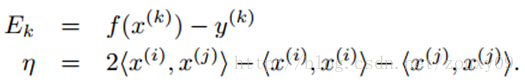
       এখানে ই কে কে-থ নমুনা হিসাবে বিবেচনা করা যেতে পারে, এসভিএমের আউটপুট এবং প্রত্যাশিত আউটপুট অর্থাৎ নমুনা লেবেলের ত্রুটি।



       এবং η আসলে আমি এবং জে দুটি নমুনার সাদৃশ্য পরিমাপ করে। Calc গণনা করার সময়, আমাদের কার্নেল ফাংশনটি ব্যবহার করা দরকার, সুতরাং আমরা উপরের অভ্যন্তরীণ পণ্যটি প্রতিস্থাপন করতে কার্নেল ফাংশনটি ব্যবহার করতে পারি।

       নতুন α j প্রাপ্ত করার পরে , আমাদের তা নিশ্চিত করা দরকার যে এটি সীমানার মধ্যে রয়েছে। অন্য কথায়, যদি এই অনুকূলিত মানটি এল এবং এইচ এর সীমানার বাইরে চলে যায় তবে আমাদের কেবল ক্রপ করে α জে এই সীমার মধ্যে ফিরিয়ে আনতে হবে :



       অবশেষে, অপ্টিমাইজ [আলফা] জে , আমরা ক্যালকুলেট [আলফা] করার জন্য এটি ব্যবহার করতে হবে আমি :



       এই মুহুর্তে, α i এবং α j এর অপ্টিমাইজেশন সম্পূর্ণ।

(3) থ্রেশহোল্ড বি গণনা করুন:

       Α i এবং α j অপ্টিমাইজ করার পরে , আমরা থ্রেশহোল্ড বি আপডেট করতে পারি যাতে কে কেটি শর্তটি আমি এবং জে উভয় নমুনার জন্য সন্তুষ্ট হয়। যদি optim i অপ্টিমাইজেশনের পরে সীমানায় না থাকে (এটি 0 <α i <C কে সন্তুষ্ট করে , তবে কেকেটি শর্ত অনুসারে আমরা y i g i (x i ) = 1 পেতে পারি, তাই আমরা খ গণনা করতে পারি), তবে নীচের প্রান্তিক মানটি বি 1 বৈধ কারণ এটি এসভিএমকে y i আউটপুট দিতে বাধ্য করে যখন x i ইনপুট থাকে ।



       একইভাবে, যদি 0 <α j <C হয় তবে নিম্নলিখিত বি 2 টিও বৈধ:



      যদি 0 <α i <C এবং 0 <α j <C সন্তুষ্ট হয় তবে বি 1 এবং বি 2 উভয়ই বৈধ এবং সেগুলি সমান। যদি উভয়ই সীমানাতে থাকে (এটি, α i = 0 বা α i = C, এবং α j = 0 বা α j = C), তবে বি 1 এবং বি 2 এর মধ্যকার প্রান্তিক কে কেটি শর্ত পূরণ করে General তাদের গড় বি = (বি 1 + বি 2) / 2। সুতরাং, সাধারণভাবে, বি-তে আপডেটটি নিম্নরূপ:



       প্রতিবার ন্যূনতম অপ্টিমাইজেশন সম্পন্ন হওয়ার পরে, পরিবর্তিত শ্রেণিবদ্ধকরণের সাথে অন্যান্য ডেটা নমুনাগুলির মুখোমুখি হওয়ার জন্য প্রতিটি ডেটা নমুনার ত্রুটি আপডেট করতে হবে এবং দ্বিতীয় জোড়যুক্ত অপ্টিমাইজড ডেটা নমুনা বাছাই করার সময় ধাপের আকারটি অনুমান করতে ব্যবহৃত হবে।

(4) উত্তল অপ্টিমাইজেশান সমস্যার জন্য সমাপ্তির শর্তাদি:

       এসএমও অ্যালগরিদমের মূল ধারণাটি: ভেরিয়েবলগুলির সাথে সমাধানগুলি যদি এই অপ্টিমাইজেশান সমস্যার কেকেটি শর্ত পূরণ করে, তবে এই অপ্টিমাইজেশন সমস্যার সমাধান পাওয়া যায়। কারণ কেকেটি শর্তটি অপ্টিমাইজেশান সমস্যার জন্য প্রয়োজনীয় এবং পর্যাপ্ত শর্ত (প্রমাণের জন্য দয়া করে রেফারেন্সটি দেখুন)। সুতরাং আমরা মূল সমস্যার কেকেটি শর্তটি পর্যবেক্ষণ করতে পারি, সুতরাং সমস্ত নমুনা কেকেটি শর্ত পূরণ করে, তারপরে পুনরাবৃত্তিটি শেষ। তবে, যেহেতু কে কেটি শর্তটি নিজেই তুলনামূলকভাবে কঠোর, এটি সহনশীলতার মানও নির্ধারণ করা প্রয়োজন, এটি হ'ল যদি সমস্ত নমুনাগুলি সহিষ্ণুতা মান সীমার মধ্যে কেকেটি শর্ত পূরণ করে তবে প্রশিক্ষণটি শেষ করা যায়; অবশ্যই, দ্বৈত সমস্যার উত্তল অপ্টিমাইজেশনের জন্য অন্যান্য সমাপ্তির শর্তাদি রয়েছে আপনি সাহিত্যের উল্লেখ করতে পারেন।



৮.৩. এসএমও অ্যালগরিদমের পাইথন বাস্তবায়ন

8.3.1 পাইথনের প্রস্তুতি

      আমি পাইথন সংস্করণটি 2.7.5 ব্যবহার করি। অতিরিক্ত লাইব্রেরি হ'ল নম্পি এবং ম্যাটপ্ল্লিটিব। ম্যাটপ্ল্লিটিব দুটি লাইব্রেরি, ডেটুটিল এবং পাইপার্সিংয়ের উপর নির্ভর করে, সুতরাং আমাদের উপরের তিনটি গ্রন্থাগার ইনস্টল করা প্রয়োজন। প্রথম দুটি গ্রন্থাগার ইনস্টল করা ঠিক আছে, এবং সম্পর্কিত সংস্করণগুলি সরাসরি অফিসিয়াল ওয়েবসাইটে ইনস্টল করা যেতে পারে। তবে আমি যখন শেষ দুটি লাইব্রেরি পেয়েছি তখন এটি এত সহজ ছিল না। পরে এটি আবিষ্কার হয়েছিল যে পাইথন গ্রন্থাগারটি পাইপ সরঞ্জামটি ব্যবহার করে ডাউনলোড এবং ইনস্টল করা যেতে পারে। পাইথন প্যাকেজ ইনস্টল ও পরিচালনা করার জন্য এটি একটি সরঞ্জাম। এটি উবুন্টুর জন্য কিছুটা উপযুক্ত মনে হয়েছে, কোন লাইব্রেরি ইনস্টল করা দরকার, সরাসরি ওয়ান স্টপ পরিষেবা ডাউনলোড এবং ইনস্টল করা উচিত।

       প্রথমত, আমাদের পাইপটির অফিসিয়াল ওয়েবসাইটে যেতে হবে: আমাদের পাইথন সংস্করণের সাথে সম্পর্কিত পাইপটি ডাউনলোড করতে https://pypi.python.org/pypi/pip , উদাহরণস্বরূপ, খনিটি পাইপ-১.৪.১.আরটি.পি.জেড। তবে পিপ ইনস্টল করার জন্য অন্য একটি সরঞ্জাম প্রয়োজন, যা সেটআপলগুলি e আমরা ez_setup.py ফাইলটি ডাউনলোড করতে https://pypi.python.org/pypi/setuptools/#windows এ গিয়ে ফিরে আসি। তারপরে সিএমডি কমান্ড লাইনে কার্যকর করুন: (তাদের পথটি নোট করুন)

#Python ez_setup.py

এই মুহুর্তে .egg এবং অন্যান্য ফাইলগুলি স্বয়ংক্রিয়ভাবে ডাউনলোড হবে এবং ইনস্টলেশনটি সম্পূর্ণ হবে।

      তারপরে আমরা পাইপ -১.৪.১.আরটি.আর.জি. এই ডিরেক্টরিতে যান এবং কার্যকর করুন:

#python setup.py ইনস্টল করুন

এই সময়ে, পাইপটি স্বয়ংক্রিয়ভাবে আপনার অজগর ডিরেক্টরিতে স্ক্রিপ্টস ফোল্ডারে ইনস্টল হবে। খনিটি সি: \ পাইথন 27 \ স্ক্রিপ্ট।

       ভিতরে আমরা পাইপ.এক্স.এই দেখতে পাব, তারপরে আমরা এই ফোল্ডারে যাব:

# সিডি সি: \ পাইথন 27 \ স্ক্রিপ্ট

# পিপ ইনস্টল ডেটুটিল

# পিপ ইনস্টল পাইপার্সিং

এটি এই অতিরিক্ত লাইব্রেরিগুলি আবার ডাউনলোড করবে। গ্রেডে খুব হাই-এন্ড পরিবেশ!

8.3.2 এসএমও অ্যালগরিদমের পাইথন বাস্তবায়ন

       কোডটিতে আরও বিস্তারিত মন্তব্য রয়েছে। কোনও ভুল আছে কিনা তা আমি জানি না so তা হলে, আমি আশা করি সবাই এগুলি সংশোধন করে (প্রতিটি রানের ফলাফল আলাদা হতে পারে In এছাড়াও, আমি মনে করি যে কিছু ফলাফল ভুল বলে মনে হচ্ছে। আপনার গাইডেন্সের জন্য আপনাকে ধন্যবাদ।) আমি ফলাফলগুলি কল্পনা করতে একটি ফাংশন লিখেছি, তবে এটি কেবলমাত্র দ্বি-মাত্রিক ডেটাতে ব্যবহার করা যেতে পারে। কোডটি সরাসরি পেস্ট করুন:

SVM.py


#################################################
# SVM: support vector machine
# Author : zouxy
# Date   : 2013-12-12
# HomePage : http://blog.csdn.net/zouxy09
# Email  : zouxy09@qq.com
#################################################

from numpy import *
import time
import matplotlib.pyplot as plt


# calulate kernel value
def calcKernelValue(matrix_x, sample_x, kernelOption):
kernelType = kernelOption[0]
numSamples = matrix_x.shape[0]
kernelValue = mat(zeros((numSamples, 1)))

if kernelType == 'linear':
kernelValue = matrix_x * sample_x.T
elif kernelType == 'rbf':
sigma = kernelOption[1]
if sigma == 0:
sigma = 1.0
for i in xrange(numSamples):
diff = matrix_x[i, :] - sample_x
kernelValue[i] = exp(diff * diff.T / (-2.0 * sigma**2))
else:
raise NameError('Not support kernel type! You can use linear or rbf!')
return kernelValue


# calculate kernel matrix given train set and kernel type
def calcKernelMatrix(train_x, kernelOption):
numSamples = train_x.shape[0]
kernelMatrix = mat(zeros((numSamples, numSamples)))
for i in xrange(numSamples):
kernelMatrix[:, i] = calcKernelValue(train_x, train_x[i, :], kernelOption)
return kernelMatrix


# define a struct just for storing variables and data
class SVMStruct:
def __init__(self, dataSet, labels, C, toler, kernelOption):
self.train_x = dataSet # each row stands for a sample
self.train_y = labels  # corresponding label
self.C = C             # slack variable
self.toler = toler     # termination condition for iteration
self.numSamples = dataSet.shape[0] # number of samples
self.alphas = mat(zeros((self.numSamples, 1))) # Lagrange factors for all samples
self.b = 0
self.errorCache = mat(zeros((self.numSamples, 2)))
self.kernelOpt = kernelOption
self.kernelMat = calcKernelMatrix(self.train_x, self.kernelOpt)


# calculate the error for alpha k
def calcError(svm, alpha_k):
output_k = float(multiply(svm.alphas, svm.train_y).T * svm.kernelMat[:, alpha_k] + svm.b)
error_k = output_k - float(svm.train_y[alpha_k])
return error_k


# update the error cache for alpha k after optimize alpha k
def updateError(svm, alpha_k):
error = calcError(svm, alpha_k)
svm.errorCache[alpha_k] = [1, error]


# select alpha j which has the biggest step
def selectAlpha_j(svm, alpha_i, error_i):
svm.errorCache[alpha_i] = [1, error_i] # mark as valid(has been optimized)
candidateAlphaList = nonzero(svm.errorCache[:, 0].A)[0] # mat.A return array
maxStep = 0; alpha_j = 0; error_j = 0

# find the alpha with max iterative step
if len(candidateAlphaList) > 1:
for alpha_k in candidateAlphaList:
if alpha_k == alpha_i:
continue
error_k = calcError(svm, alpha_k)
if abs(error_k - error_i) > maxStep:
maxStep = abs(error_k - error_i)
alpha_j = alpha_k
error_j = error_k
# if came in this loop first time, we select alpha j randomly
else:       
alpha_j = alpha_i
while alpha_j == alpha_i:
alpha_j = int(random.uniform(0, svm.numSamples))
error_j = calcError(svm, alpha_j)

return alpha_j, error_j


# the inner loop for optimizing alpha i and alpha j
def innerLoop(svm, alpha_i):
error_i = calcError(svm, alpha_i)

### check and pick up the alpha who violates the KKT condition
## satisfy KKT condition
# 1) yi*f(i) >= 1 and alpha == 0 (outside the boundary)
# 2) yi*f(i) == 1 and 0<alpha< C (on the boundary)
# 3) yi*f(i) <= 1 and alpha == C (between the boundary)
## violate KKT condition
# because y[i]*E_i = y[i]*f(i) - y[i]^2 = y[i]*f(i) - 1, so
# 1) if y[i]*E_i < 0, so yi*f(i) < 1, if alpha < C, violate!(alpha = C will be correct)
# 2) if y[i]*E_i > 0, so yi*f(i) > 1, if alpha > 0, violate!(alpha = 0 will be correct)
# 3) if y[i]*E_i = 0, so yi*f(i) = 1, it is on the boundary, needless optimized
if (svm.train_y[alpha_i] * error_i < -svm.toler) and (svm.alphas[alpha_i] < svm.C) or\
(svm.train_y[alpha_i] * error_i > svm.toler) and (svm.alphas[alpha_i] > 0):

# step 1: select alpha j
alpha_j, error_j = selectAlpha_j(svm, alpha_i, error_i)
alpha_i_old = svm.alphas[alpha_i].copy()
alpha_j_old = svm.alphas[alpha_j].copy()

# step 2: calculate the boundary L and H for alpha j
if svm.train_y[alpha_i] != svm.train_y[alpha_j]:
L = max(0, svm.alphas[alpha_j] - svm.alphas[alpha_i])
H = min(svm.C, svm.C + svm.alphas[alpha_j] - svm.alphas[alpha_i])
else:
L = max(0, svm.alphas[alpha_j] + svm.alphas[alpha_i] - svm.C)
H = min(svm.C, svm.alphas[alpha_j] + svm.alphas[alpha_i])
if L == H:
return 0

# step 3: calculate eta (the similarity of sample i and j)
eta = 2.0 * svm.kernelMat[alpha_i, alpha_j] - svm.kernelMat[alpha_i, alpha_i] \
  - svm.kernelMat[alpha_j, alpha_j]
if eta >= 0:
return 0

# step 4: update alpha j
svm.alphas[alpha_j] -= svm.train_y[alpha_j] * (error_i - error_j) / eta

# step 5: clip alpha j
if svm.alphas[alpha_j] > H:
svm.alphas[alpha_j] = H
if svm.alphas[alpha_j] < L:
svm.alphas[alpha_j] = L

# step 6: if alpha j not moving enough, just return
if abs(alpha_j_old - svm.alphas[alpha_j]) < 0.00001:
updateError(svm, alpha_j)
return 0

# step 7: update alpha i after optimizing aipha j
svm.alphas[alpha_i] += svm.train_y[alpha_i] * svm.train_y[alpha_j] \
* (alpha_j_old - svm.alphas[alpha_j])

# step 8: update threshold b
b1 = svm.b - error_i - svm.train_y[alpha_i] * (svm.alphas[alpha_i] - alpha_i_old) \
* svm.kernelMat[alpha_i, alpha_i] \
- svm.train_y[alpha_j] * (svm.alphas[alpha_j] - alpha_j_old) \
* svm.kernelMat[alpha_i, alpha_j]
b2 = svm.b - error_j - svm.train_y[alpha_i] * (svm.alphas[alpha_i] - alpha_i_old) \
* svm.kernelMat[alpha_i, alpha_j] \
- svm.train_y[alpha_j] * (svm.alphas[alpha_j] - alpha_j_old) \
* svm.kernelMat[alpha_j, alpha_j]
if (0 < svm.alphas[alpha_i]) and (svm.alphas[alpha_i] < svm.C):
svm.b = b1
elif (0 < svm.alphas[alpha_j]) and (svm.alphas[alpha_j] < svm.C):
svm.b = b2
else:
svm.b = (b1 + b2) / 2.0

# step 9: update error cache for alpha i, j after optimize alpha i, j and b
updateError(svm, alpha_j)
updateError(svm, alpha_i)

return 1
else:
return 0


# the main training procedure
def trainSVM(train_x, train_y, C, toler, maxIter, kernelOption = ('rbf', 1.0)):
# calculate training time
startTime = time.time()

# init data struct for svm
svm = SVMStruct(mat(train_x), mat(train_y), C, toler, kernelOption)

# start training
entireSet = True
alphaPairsChanged = 0
iterCount = 0
# Iteration termination condition:
# Condition 1: reach max iteration
# Condition 2: no alpha changed after going through all samples,
# in other words, all alpha (samples) fit KKT condition
while (iterCount < maxIter) and ((alphaPairsChanged > 0) or entireSet):
alphaPairsChanged = 0

# update alphas over all training examples
if entireSet:
for i in xrange(svm.numSamples):
alphaPairsChanged += innerLoop(svm, i)
print '---iter:%d entire set, alpha pairs changed:%d' % (iterCount, alphaPairsChanged)
iterCount += 1
# update alphas over examples where alpha is not 0 & not C (not on boundary)
else:
nonBoundAlphasList = nonzero((svm.alphas.A > 0) * (svm.alphas.A < svm.C))[0]
for i in nonBoundAlphasList:
alphaPairsChanged += innerLoop(svm, i)
print '---iter:%d non boundary, alpha pairs changed:%d' % (iterCount, alphaPairsChanged)
iterCount += 1

# alternate loop over all examples and non-boundary examples
if entireSet:
entireSet = False
elif alphaPairsChanged == 0:
entireSet = True

print 'Congratulations, training complete! Took %fs!' % (time.time() - startTime)
return svm


# testing your trained svm model given test set
def testSVM(svm, test_x, test_y):
test_x = mat(test_x)
test_y = mat(test_y)
numTestSamples = test_x.shape[0]
supportVectorsIndex = nonzero(svm.alphas.A > 0)[0]
supportVectors = svm.train_x[supportVectorsIndex]
supportVectorLabels = svm.train_y[supportVectorsIndex]
supportVectorAlphas = svm.alphas[supportVectorsIndex]
matchCount = 0
for i in xrange(numTestSamples):
kernelValue = calcKernelValue(supportVectors, test_x[i, :], svm.kernelOpt)
predict = kernelValue.T * multiply(supportVectorLabels, supportVectorAlphas) + svm.b
if sign(predict) == sign(test_y[i]):
matchCount += 1
accuracy = float(matchCount) / numTestSamples
return accuracy


# show your trained svm model only available with 2-D data
def showSVM(svm):
if svm.train_x.shape[1] != 2:
print "Sorry! I can not draw because the dimension of your data is not 2!"
return 1

# draw all samples
for i in xrange(svm.numSamples):
if svm.train_y[i] == -1:
plt.plot(svm.train_x[i, 0], svm.train_x[i, 1], 'or')
elif svm.train_y[i] == 1:
plt.plot(svm.train_x[i, 0], svm.train_x[i, 1], 'ob')

# mark support vectors
supportVectorsIndex = nonzero(svm.alphas.A > 0)[0]
for i in supportVectorsIndex:
plt.plot(svm.train_x[i, 0], svm.train_x[i, 1], 'oy')

# draw the classify line
w = zeros((2, 1))
for i in supportVectorsIndex:
w += multiply(svm.alphas[i] * svm.train_y[i], svm.train_x[i, :].T)
min_x = min(svm.train_x[:, 0])[0, 0]
max_x = max(svm.train_x[:, 0])[0, 0]
y_min_x = float(-svm.b - w[0] * min_x) / w[1]
y_max_x = float(-svm.b - w[0] * max_x) / w[1]
plt.plot([min_x, max_x], [y_min_x, y_max_x], '-g')
plt.show()

       পরীক্ষা থেকে ডেটা এখানে । এখানে 100 টি নমুনা রয়েছে, প্রতিটি নমুনা দ্বি-মাত্রিক এবং সংশ্লিষ্ট লেবেলটি শেষে থাকে, উদাহরণস্বরূপ:

3.542485 1.977398 -1

3.018896 2.556416 -1

7.551510 -1.580030 1

2.114999 -0.004466 -1

......

       পরীক্ষার কোডটি প্রথমে এই ডাটাবেসটি লোড করে, তারপরে প্রশিক্ষণের জন্য প্রথম 80 টি নমুনা ব্যবহার করে এবং তারপরে পরীক্ষার জন্য অবশিষ্ট 20 টি নমুনা ব্যবহার করে এবং প্রশিক্ষিত মডেল এবং শ্রেণিবিন্যাসের ফলাফলগুলি প্রদর্শন করে। পরীক্ষার কোডটি নিম্নরূপ:

test_SVM.py


#################################################
# SVM: support vector machine
# Author : zouxy
# Date   : 2013-12-12
# HomePage : http://blog.csdn.net/zouxy09
# Email  : zouxy09@qq.com
#################################################

from numpy import *
import SVM

################## test svm #####################
## step 1: load data
print "step 1: load data..."
dataSet = []
labels = []
fileIn = open('E:/Python/Machine Learning in Action/testSet.txt')
for line in fileIn.readlines():
lineArr = line.strip().split('\t')
dataSet.append([float(lineArr[0]), float(lineArr[1])])
labels.append(float(lineArr[2]))

dataSet = mat(dataSet)
labels = mat(labels).T
train_x = dataSet[0:81, :]
train_y = labels[0:81, :]
test_x = dataSet[80:101, :]
test_y = labels[80:101, :]

## step 2: training...
print "step 2: training..."
C = 0.6
toler = 0.001
maxIter = 50
svmClassifier = SVM.trainSVM(train_x, train_y, C, toler, maxIter, kernelOption = ('linear', 0))

## step 3: testing
print "step 3: testing..."
accuracy = SVM.testSVM(svmClassifier, test_x, test_y)

## step 4: show the result
print "step 4: show the result..."
print 'The classify accuracy is: %.3f%%' % (accuracy * 100)
SVM.showSVM(svmClassifier)

ফলাফলগুলি নিম্নরূপ:


step 1: load data...
step 2: training...
---iter:0 entire set, alpha pairs changed:8
---iter:1 non boundary, alpha pairs changed:7
---iter:2 non boundary, alpha pairs changed:1
---iter:3 non boundary, alpha pairs changed:0
---iter:4 entire set, alpha pairs changed:0
Congratulations, training complete! Took 0.058000s!
step 3: testing...
step 4: show the result...
The classify accuracy is: 100.000%

প্রশিক্ষিত মডেল ডায়াগ্রাম: