Interpretation of multi-granular cascade forest
This blog post briefly explains Professor Zhou Zhihua's multi-granular cascade forest algorithm. Not much nonsense, the structure of a multi-granular cascade forest is mainly divided into two parts, one is the multi-granular scanning part, and the other is the cascade forest part. The multi-granularity scan structure diagram is shown below:
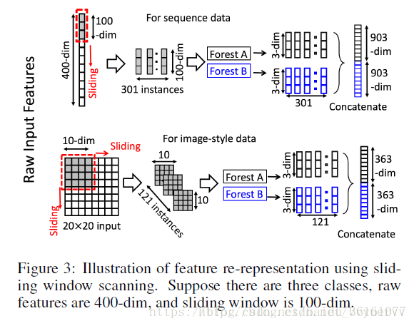
As can be seen from the above figure, assuming that the original data is 400-dimensional, and then sliding with a slider size of 100,200,300, respectively, to obtain 301 * 100, 201 * 100, 101 * 100 data, that is, 301, 201, 101 The examples are 100-dimensional, 200-dimensional, and 300-dimensional sub-sample data. These data are actually features in one sample. There are not 301 samples. However, for the sake of understanding, these 301 are used as sub-samples. This step is a bit of k-fold cross sampling, and then send this batch of data to the cascaded random forest. The random forests here appear in pairs, one is the ordinary random forest, and the other is a completely random forest. In order to increase the ensemble learning Diversity. The difference between completely random forests and ordinary random forests is that each tree in a completely random forest is generated by randomly selecting a feature at each node of the tree to achieve segmentation, and the tree continues to grow until each leaf node contains only the same class of Examples or no more than 10 examples. Similarly, each common random forest trees 1000 also include, by random selection √(d)
The number of features are candidates (d is the number of input features), and then the feature with the best gini value is selected as the segmentation. The value of the tree in each forest is a hyperparameter. Assume that the number of categories after classification of a random forest is 3. After a sample passes a random forest, a 3-dimensional probability distribution is obtained. Previously, we obtained 301, 201, and 101 samples, respectively. Then these 3 batches of samples enter a random forest In the future, there are 903,603,303 probabilities. In the figure, 2 random forests are used for each batch, then the number of probabilities finally obtained is 903 X 2, 603 X 2, 303 X 2. Then these probabilities are obtained. The stitching is called one, and it becomes a data of 3618dim. At this point, the step of multi-granularity scanning is completed. The process of multi-granularity scanning is equivalent to the extraction of features. The following is the process of cascading forests.
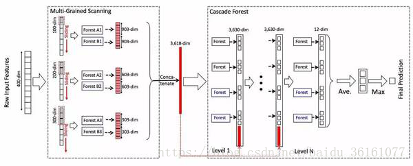
Send the 3618-dimensional data x to the random forest, and each random forest gets a 3-dimensional data. In the figure, 4 random forests are used, of which the two black ones are completely random forests. Two of them are ordinary random forests. In this way, four 3-dimensional density data are obtained. Then the original x is stitched together to become 3618 + 12 = 3630-dimensional data. This data is used as the next layer. Input, and then get 4 three-dimensional data, and then stitch with the original x to obtain 3630-dimensional surgical data, as the input of the next layer, so that it is passed to the last layer, and the original data need not be stitched together again. , Because it is the last layer, there is no need to stitch it together as the input of the next layer, and finally output 4 3D data, average the 4 3D data to get a 3D data, and then Take the largest one in this 3-dimensional data as a prediction. The number of layers in the entire multi-granular cascade forest is adaptively adjusted. During the construction phase of the cascade forest, as long as the current layer is constructed, the cross-validation verification accuracy is not improved compared to the previous layer. Construction stopped and the entire structure was completed.
Well, the basic algorithm structure has been roughly analyzed, and it will be gradually improved later, such as the composition of random forests, attribute split measurement methods in decision trees, and so on. It's time for dinner. . . . . . . . . . . . . .
#!usr/bin/env python
"""
Version : 0.1.4
Date : 15th April 2017
Author : Pierre-Yves Lablanche
Email : plablanche@aims.ac.za
Affiliation : African Institute for Mathematical Sciences - South Africa
Stellenbosch University - South Africa
License : MIT
Status : Under Development
Description :
Python3 implementation of the gcForest algorithm preesented in Zhou and Feng 2017
(paper can be found here : https://arxiv.org/abs/1702.08835 ).
It uses the typical scikit-learn syntax with a .fit() function for training
and a .predict() function for predictions.
"""
import itertools
import numpy as np
from sklearn.ensemble import RandomForestClassifier
from sklearn.model_selection import train_test_split
from sklearn.metrics import accuracy_score
__author__ = "Pierre-Yves Lablanche"
__email__ = "plablanche@aims.ac.za"
__license__ = "MIT"
__version__ = "0.1.4"
__status__ = "Development"
# noinspection PyUnboundLocalVariable
class gcForest(object):
def __init__(self, shape_1X=None, n_mgsRFtree=30, window=None, stride=1,
cascade_test_size=0.2, n_cascadeRF=2, n_cascadeRFtree=101, cascade_layer=np.inf,
min_samples_mgs=0.1, min_samples_cascade=0.05, tolerance=0.0, n_jobs=1):
'''
shape_1X:单个样本元素的形状,可以是int型的数字、元组、列表形式
n_mgsRFtree: 多粒度扫描时,随机森林中的决策树的个数,多粒度扫描阶段的决策树的个数30
window:滑动窗口
stride:滑动步长
cascade_test_size:测试集占总共几个的分数或者测试集的样本的个数
n_cascadeRF: 一个级联层中的随机森林的个数,每个完全随机森林对应了一个普通随机森林(伪随机森林)
所以一个级联层中的随机森林的个数是 2 × n_cascadeRF
n_cascadeRFtree:级联森林中单个随机森林中决策树的个数101
tolerance 如果级联森林中一级一级往下传递下去的时候,精确度的提升不再大于tolerance,那么cascade_layer就不再增长了,就停止了
n_jobs 是并行处理的随机森林的个数,在RandomForestClassifier中有n_jobs 这个参数
'''
""" gcForest Classifier.
:param shape_1X: int or tuple list or np.array (default=None)
Shape of a single sample element [n_lines, n_cols]. Required when calling mg_scanning!
For sequence data a single int can be given.
:param n_mgsRFtree: int (default=30)
Number of trees in a Random Forest during Multi Grain Scanning.
:param window: int (default=None)
List of window sizes to use during Multi Grain Scanning.
If 'None' no slicing will be done.
:param stride: int (default=1)
Step used when slicing the data.
:param cascade_test_size: float or int (default=0.2)
Split fraction or absolute number for cascade training set splitting.
:param n_cascadeRF: int (default=2)
Number of Random Forests in a cascade layer.
For each pseudo Random Forest a complete Random Forest is created, hence
the total numbe of Random Forests in a layer will be 2*n_cascadeRF.
:param n_cascadeRFtree: int (default=101)
Number of trees in a single Random Forest in a cascade layer.
:param min_samples_mgs: float or int (default=0.1)
Minimum number of samples in a node to perform a split
during the training of Multi-Grain Scanning Random Forest.
If int number_of_samples = int.
If float, min_samples represents the fraction of the initial n_samples to consider.
:param min_samples_cascade: float or int (default=0.1)
Minimum number of samples in a node to perform a split
during the training of Cascade Random Forest.
If int number_of_samples = int.
If float, min_samples represents the fraction of the initial n_samples to consider.
:param cascade_layer: int (default=np.inf)
mMximum number of cascade layers allowed.
Useful to limit the contruction of the cascade.
:param tolerance: float (default=0.0)
Accuracy tolerance for the casacade growth.
If the improvement in accuracy is not better than the tolerance the construction is
stopped.
:param n_jobs: int (default=1)
The number of jobs to run in parallel for any Random Forest fit and predict.
If -1, then the number of jobs is set to the number of cores.
"""
setattr(self, 'shape_1X', shape_1X)
setattr(self, 'n_layer', 0)
setattr(self, '_n_samples', 0)
setattr(self, 'n_cascadeRF', int(n_cascadeRF))
if isinstance(window, int):
#这里的if elif 是为了将window 处理成列表的形式
setattr(self, 'window', [window])
elif isinstance(window, list):
setattr(self, 'window', window)
setattr(self, 'stride', stride)
setattr(self, 'cascade_test_size', cascade_test_size)
setattr(self, 'n_mgsRFtree', int(n_mgsRFtree))
setattr(self, 'n_cascadeRFtree', int(n_cascadeRFtree))
setattr(self, 'cascade_layer', cascade_layer)
setattr(self, 'min_samples_mgs', min_samples_mgs)
setattr(self, 'min_samples_cascade', min_samples_cascade)
setattr(self, 'tolerance', tolerance)
setattr(self, 'n_jobs', n_jobs)
def fit(self, X, y):
""" Training the gcForest on input data X and associated target y.
:param X: np.array
Array containing the input samples.
Must be of shape [n_samples, data] where data is a 1D array.
:param y: np.array
1D array containing the target values.
Must be of shape [n_samples]
"""
if np.shape(X)[0] != len(y):
raise ValueError('Sizes of y and X do not match.')
mgs_X = self.mg_scanning(X, y)
_ = self.cascade_forest(mgs_X, y)
def predict_proba(self, X):
""" Predict the class probabilities of unknown samples X.
:param X: np.array
Array containing the input samples.
Must be of the same shape [n_samples, data] as the training inputs.
:return: np.array
1D array containing the predicted class probabilities for each input sample.
"""
mgs_X = self.mg_scanning(X)
cascade_all_pred_prob = self.cascade_forest(mgs_X)
predict_proba = np.mean(cascade_all_pred_prob, axis=0)
return predict_proba
def predict(self, X):
""" Predict the class of unknown samples X.
:param X: np.array
Array containing the input samples.
Must be of the same shape [n_samples, data] as the training inputs.
:return: np.array
1D array containing the predicted class for each input sample.
"""
pred_proba = self.predict_proba(X=X)
predictions = np.argmax(pred_proba, axis=1)
return predictions
def mg_scanning(self, X, y=None):
""" Performs a Multi Grain Scanning on input data.
:param X: np.array
Array containing the input samples.
Must be of shape [n_samples, data] where data is a 1D array.
:param y: np.array (default=None)
:return: np.array
Array of shape [n_samples, .. ] containing Multi Grain Scanning sliced data.
"""
setattr(self, '_n_samples', np.shape(X)[0]) #样本的个数
shape_1X = getattr(self, 'shape_1X') # 单个样本元素的形状
if isinstance(shape_1X, int):
# 如果shape_1X是int型的数据如,就给它加个维度
#单个样本的形状就变成了[1,shape_1X],如果shape_1X是3,那么后面就会变成[1,3]的形状,
#像[1,3]这样的数据是属于时序数据
shape_1X = [1,shape_1X]
if not getattr(self, 'window'):
setattr(self, 'window', [shape_1X[1]])
'''
这里的window是列表的形式,在论文中分别取了[100,200,300]的大小的窗口,在下面的代码中,会将
不同大小的窗口一个个取出来(int型),然后用这些大小不同的窗口去扫描原始数据。下面的win_size
就是传到方法中的参数window,上面的window 和下面的window 类型不是一样的
'''
mgs_pred_prob = [] #多粒度扫描输出的三个概率就存在这个列表里面
for wdw_size in getattr(self, 'window'): #在多粒度扫描阶段,论文的图中用了3种不同的滑动窗口
#分别是100,200,300大小的
wdw_pred_prob = self.window_slicing_pred_prob(X, wdw_size, shape_1X, y=y)#扫描
mgs_pred_prob.append(wdw_pred_prob)
return np.concatenate(mgs_pred_prob, axis=1)
def window_slicing_pred_prob(self, X, window, shape_1X, y=None):
""" Performs a window slicing of the input data and send them through Random Forests.
If target values 'y' are provided sliced data are then used to train the Random Forests.
:param X: np.array
Array containing the input samples.
Must be of shape [n_samples, data] where data is a 1D array.
:param window: int
Size of the window to use for slicing.
:param shape_1X: list or np.array
Shape of a single sample.
:param y: np.array (default=None)
Target values. If 'None' no training is done.
:return: np.array
Array of size [n_samples, ..] containing the Random Forest.
prediction probability for each input sample.
"""
n_tree = getattr(self, 'n_mgsRFtree')#每个随机森林中决策树的个数
min_samples = getattr(self, 'min_samples_mgs')#多粒度扫描时最小的样本数或者最小占比0.1
stride = getattr(self, 'stride')# 步长
if shape_1X[0] > 1:# 如果样本数组的行数大于1,可以判断为是图像数据
print('Slicing Images...')
sliced_X, sliced_y = self._window_slicing_img(X, window, shape_1X, y=y, stride=stride)# 图像扫描
else:#否则就是时序数据
print('Slicing Sequence...')
sliced_X, sliced_y = self._window_slicing_sequence(X, window, shape_1X, y=y, stride=stride)#时序数据扫描
if y is not None:#当样本有标签时
n_jobs = getattr(self, 'n_jobs')# 0
#扫描完成后进入随机森林,经过随机森林后得到3维的数据
prf = RandomForestClassifier(n_estimators=n_tree, max_features='sqrt',
min_samples_split=min_samples, oob_score=True, n_jobs=n_jobs)
# 搭建随机森林框架
crf = RandomForestClassifier(n_estimators=n_tree, max_features=None,
min_samples_split=min_samples, oob_score=True, n_jobs=n_jobs)
print('Training MGS Random Forests...')
prf.fit(sliced_X, sliced_y)# 将扫描得到的数据送到随机森林里面,随机森林有两种
crf.fit(sliced_X, sliced_y)# crf是普通随机森林 common
setattr(self, '_mgsprf_{}'.format(window), prf)
setattr(self, '_mgscrf_{}'.format(window), crf)
pred_prob_prf = prf.oob_decision_function_
pred_prob_crf = crf.oob_decision_function_
if hasattr(self, '_mgsprf_{}'.format(window)) and y is None:
prf = getattr(self, '_mgsprf_{}'.format(window))
crf = getattr(self, '_mgscrf_{}'.format(window))
pred_prob_prf = prf.predict_proba(sliced_X)
pred_prob_crf = crf.predict_proba(sliced_X)
pred_prob = np.c_[pred_prob_prf, pred_prob_crf]
return pred_prob.reshape([getattr(self, '_n_samples'), -1])
def _window_slicing_img(self, X, window, shape_1X, y=None, stride=1):
""" Slicing procedure for images
:param X: np.array
Array containing the input samples.
Must be of shape [n_samples, data] where data is a 1D array.
:param window: int
Size of the window to use for slicing.
:param shape_1X: list or np.array
Shape of a single sample [n_lines, n_cols].
:param y: np.array (default=None)
Target values.
:param stride: int (default=1)
Step used when slicing the data.
:return: np.array and np.array
Arrays containing the sliced images and target values (empty if 'y' is None).
"""
if any(s < window for s in shape_1X):
#图像数据的两个维度都小于窗口的大小,那就报错
raise ValueError('window must be smaller than both dimensions for an image')
len_iter_x = np.floor_divide((shape_1X[1] - window), stride) + 1#属性方向滑块滑动之后得到的维度
#假设图片为20X20,滑块大小为10x10,步长为1,滑动之后得到的维度就是len = (20 - 10) / 1 + 1 = 11
len_iter_y = np.floor_divide((shape_1X[0] - window), stride) + 1
iterx_array = np.arange(0, stride*len_iter_x, stride)
itery_array = np.arange(0, stride*len_iter_y, stride)
ref_row = np.arange(0, window)#这里传进来的window是一个int型数据
ref_ind = np.ravel([ref_row + shape_1X[1] * i for i in range(window)])
inds_to_take = [ref_ind + ix + shape_1X[1] * iy
for ix, iy in itertools.product(iterx_array, itery_array)]
#index to take 取的像素点索引
'''
如果图像的像素点的位置可以用数字来表示的话.比如一张图片的像素是 15X15,用5X5的滑动块
来取图片的像素,那么得到的索引就是[[array([0,1,2,3,4,15,16,17,18,19,30,31,32,
33,34,45,46,47,48,49,60,61,62,63,64,65]),array(......)]],这组数字就代表了
需要被卷积出来的像素点的位置,一行有15个,第一行是0 -- 14,最后一行是第15行,最后一个
像素点的索引号是15 ** 2 - 1 = 244
'''
sliced_imgs = np.take(X, inds_to_take, axis=1).reshape(-1, window**2)
#列向取像素点,将取到的像素点展平,再重新弄成窗口的大小: window ** 2
#shape_1X是列表,只包含两个元素[len(row),len(column)],X是原始图片
sliced_target = np.repeat(y, len_iter_x * len_iter_y)
'''
这里的y是label,上面我们用类似卷积的方式从图像中获得了特征信息,横向走了len_iter_x次,
列向走了len_iter_y次,这样我们就总共的到了36个像素块,每个像素块的大小都是window * window的
我们将每块像素块都赋予标签信息,为了后面随机森林的拟合,repeat是复制
'''
return sliced_imgs, sliced_target
def _window_slicing_sequence(self, X, window, shape_1X, y=None, stride=1):
""" Slicing procedure for sequences (aka shape_1X = [.., 1]).
:param X: np.array
Array containing the input samples.
Must be of shape [n_samples, data] where data is a 1D array.
:param window: int
Size of the window to use for slicing.
:param shape_1X: list or np.array
Shape of a single sample [n_lines, n_col].
:param y: np.array (default=None)
Target values.
:param stride: int (default=1)
Step used when slicing the data.
:return: np.array and np.array
Arrays containing the sliced sequences and target values (empty if 'y' is None).
"""
if shape_1X[1] < window:
raise ValueError('window must be smaller than the sequence dimension')
len_iter = np.floor_divide((shape_1X[1] - window), stride) + 1
iter_array = np.arange(0, stride*len_iter, stride)
ind_1X = np.arange(np.prod(shape_1X))
inds_to_take = [ind_1X[i:i+window] for i in iter_array]
sliced_sqce = np.take(X, inds_to_take, axis=1).reshape(-1, window)
sliced_target = np.repeat(y, len_iter)
return sliced_sqce, sliced_target
def cascade_forest(self, X, y=None):# 级联森林阶段
""" Perform (or train if 'y' is not None) a cascade forest estimator.
:param X: np.array
Array containing the input samples.
Must be of shape [n_samples, data] where data is a 1D array.
:param y: np.array (default=None)
Target values. If 'None' perform training.
:return: np.array
1D array containing the predicted class for each input sample.
"""
if y is not None:# if y is not None,表示的就是进入训练阶段,测试阶段送到forest是不需要送label的
setattr(self, 'n_layer', 0)
test_size = getattr(self, 'cascade_test_size')# 0.2 测试集占数据集的比例
max_layers = getattr(self, 'cascade_layer') # cascade_layer = np.inf
#这里用了最大的网络深度是无限大,就是让网络自己调整深度,等到精度增长不再变化了,因为此代码中的tolerance = 0
tol = getattr(self, 'tolerance')
X_train, X_test, y_train, y_test = train_test_split(X, y, test_size=test_size)
self.n_layer += 1
prf_crf_pred_ref = self._cascade_layer(X_train, y_train)
accuracy_ref = self._cascade_evaluation(X_test, y_test)
feat_arr = self._create_feat_arr(X_train, prf_crf_pred_ref)#传进来的原始数据集和经过随机森林后得到的概率向量拼接
self.n_layer += 1
prf_crf_pred_layer = self._cascade_layer(feat_arr, y_train)
accuracy_layer = self._cascade_evaluation(X_test, y_test)#准确度提升
while accuracy_layer > (accuracy_ref + tol) and self.n_layer <= max_layers:
accuracy_ref = accuracy_layer
prf_crf_pred_ref = prf_crf_pred_layer
feat_arr = self._create_feat_arr(X_train, prf_crf_pred_ref)
self.n_layer += 1
prf_crf_pred_layer = self._cascade_layer(feat_arr, y_train)
accuracy_layer = self._cascade_evaluation(X_test, y_test)
elif y is None:
at_layer = 1
prf_crf_pred_ref = self._cascade_layer(X, layer=at_layer)
while at_layer < getattr(self, 'n_layer'):
at_layer += 1
feat_arr = self._create_feat_arr(X, prf_crf_pred_ref)
prf_crf_pred_ref = self._cascade_layer(feat_arr, layer=at_layer)
return prf_crf_pred_ref
def _cascade_layer(self, X, y=None, layer=0):
""" Cascade layer containing Random Forest estimators.
If y is not None the layer is trained.
:param X: np.array
Array containing the input samples.
Must be of shape [n_samples, data] where data is a 1D array.
:param y: np.array (default=None)
Target values. If 'None' perform training.
:param layer: int (default=0)
Layer indice. Used to call the previously trained layer.
:return: list
List containing the prediction probabilities for all samples.
"""
n_tree = getattr(self, 'n_cascadeRFtree')# 101 级联森林中每个随机森林中决策树的个数
n_cascadeRF = getattr(self, 'n_cascadeRF') # 2
min_samples = getattr(self, 'min_samples_cascade') # 0
n_jobs = getattr(self, 'n_jobs') # 0
prf = RandomForestClassifier(n_estimators=n_tree, max_features='sqrt',
min_samples_split=min_samples, oob_score=True, n_jobs=n_jobs) # 普通随机森林
crf = RandomForestClassifier(n_estimators=n_tree, max_features=None,
min_samples_split=min_samples, oob_score=True, n_jobs=n_jobs)
# 上面的prf 和 crf只是搭建好了随机森林的框架,并没有送入数据
prf_crf_pred = []
if y is not None:# 有标签label
print('Adding/Training Layer, n_layer={}'.format(self.n_layer))
for irf in range(n_cascadeRF):
prf.fit(X, y)
crf.fit(X, y)
setattr(self, '_casprf{}_{}'.format(self.n_layer, irf), prf)
#指明prf,crf是级联森林中的那一层的随机森林的prf和crf
setattr(self, '_cascrf{}_{}'.format(self.n_layer, irf), crf)
prf_crf_pred.append(prf.oob_decision_function_)
prf_crf_pred.append(crf.oob_decision_function_)
elif y is None:# 无标签
for irf in range(n_cascadeRF):
prf = getattr(self, '_casprf{}_{}'.format(layer, irf))
crf = getattr(self, '_cascrf{}_{}'.format(layer, irf))
prf_crf_pred.append(prf.predict_proba(X))
prf_crf_pred.append(crf.predict_proba(X))
return prf_crf_pred#得到的是经过每个随机森林后得到的一个3维概率向量的拼接
def _cascade_evaluation(self, X_test, y_test): # 计算准确率
""" Evaluate the accuracy of the cascade using X and y.
:param X_test: np.array
Array containing the test input samples.
Must be of the same shape as training data.
:param y_test: np.array
Test target values.
:return: float
the cascade accuracy.
"""
casc_pred_prob = np.mean(self.cascade_forest(X_test), axis=0)
casc_pred = np.argmax(casc_pred_prob, axis=1)
casc_accuracy = accuracy_score(y_true=y_test, y_pred=casc_pred)
print('Layer validation accuracy = {}'.format(casc_accuracy))
return casc_accuracy
def _create_feat_arr(self, X, prf_crf_pred):
""" Concatenate the original feature vector with the predicition probabilities
of a cascade layer.
向量拼接,将原始的x和经过随机森立后得到的向量进行拼接
:param X: np.array
Array containing the input samples.
Must be of shape [n_samples, data] where data is a 1D array.
:param prf_crf_pred: list
Prediction probabilities by a cascade layer for X.
:return: np.array
Concatenation of X and the predicted probabilities.
To be used for the next layer in a cascade forest.
"""
swap_pred = np.swapaxes(prf_crf_pred, 0, 1)
add_feat = swap_pred.reshape([np.shape(X)[0], -1])
feat_arr = np.concatenate([add_feat, X], axis=1)
return feat_arr
(1 to 499)
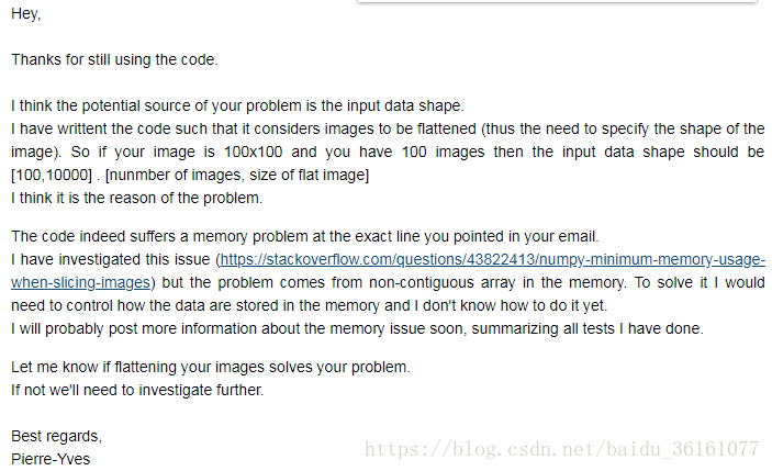
After my own test, the code of this algorithm is excellent in memory, because in the multi-granularity scanning part, through multi-granularity scanning, it is equivalent to fully extracting the characteristics of the sample, but at the same time it brings the increase of sub-samples and also brings To calculate the skyrocketing memory. At present, the code is not suitable for data with too large dimensions or data with large sample sizes, although the algorithm is originally designed for small samples. And this code can only be used for image data of a single channel, not for image data of multiple channels. In addition, the PY people who write this code are very good, and they have to answer any questions. You can ask questions.
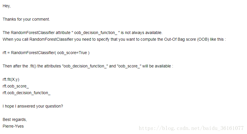
The above diagrams are some of the flaws in the code, and the reader can make corresponding research and adjustments as needed.
এই ব্লগ পোস্টটি সংক্ষেপে অধ্যাপক ঝো ঝিহুয়ার বহু-দানাদার ক্যাসকেড ফরেস্ট অ্যালগরিদমকে ব্যাখ্যা করেছে explains খুব বাজে কথা নয়, বহু-দানাদার ক্যাসকেড অরণ্যের কাঠামোটি মূলত দুটি অংশে বিভক্ত, একটি হ'ল মাল্টি-গ্রানুলার স্ক্যানিং অংশ এবং অন্যটি ক্যাসকেড বনাঞ্চল। মাল্টি-গ্রানুলারিটি স্ক্যান স্ট্রাকচার চিত্রটি নীচে দেখানো হয়েছে:
উপরের চিত্র থেকে দেখা যাবে, ধরে নেওয়া যায় যে মূল তথ্যটি 400-মাত্রিক, এবং তারপরে 301 * 100, 201 * 100, 101 * 100 ডেটা প্রাপ্ত করার জন্য যথাক্রমে 100,200,300 এর স্লাইডার আকার সহ স্লাইডিং, অর্থাৎ 301 , 201, 101 উদাহরণগুলি 100-মাত্রিক, 200-মাত্রিক এবং 300-মাত্রিক উপ-নমুনা ডেটা। এই তথ্যগুলি আসলে একটি নমুনায় বৈশিষ্ট্যযুক্ত। 301 নমুনা নেই। যাইহোক, বোঝার স্বার্থে, এই 301 টি উপ-নমুনা হিসাবে ব্যবহৃত হয়। এই পদক্ষেপটি কিছুটা কে-ফোল্ড ক্রস স্যাম্পলিং, এবং তারপরে এই ব্যাচের ডেটাটি ক্যাসকেড এলোমেলো বনের কাছে প্রেরণ করুন। এলোমেলো বন এখানে জোড়াতে উপস্থিত হয়, একটি হ'ল সাধারণ এলোমেলো বন এবং অন্যটি সম্পূর্ণ র্যান্ডম বন। যাতে নকশাকরণ শেখার বৈচিত্র্য বাড়ানো যায়। সম্পূর্ণ এলোমেলো বন এবং সাধারণ এলোমেলো বনের মধ্যে পার্থক্য হ'ল সম্পূর্ণ র্যান্ডম বনের প্রতিটি গাছ বিভাজন অর্জনের জন্য এলোমেলোভাবে গাছের প্রতিটি নোডে একটি বৈশিষ্ট্য নির্বাচন করে উত্পন্ন হয় এবং প্রতিটি পাতার নোডে কেবল একই থাকে না হওয়া পর্যন্ত গাছটি বাড়তে থাকে উদাহরণগুলির শ্রেণি বা 10 টির বেশি উদাহরণ নয়। একইভাবে, প্রতিটি সাধারণ এলোমেলো বন গাছগুলিও এলোমেলোভাবে নির্বাচনের মাধ্যমে অন্তর্ভুক্ত থাকে rut (d) বৈশিষ্ট্যগুলির সংখ্যা প্রার্থী হয় (ডি ইনপুট বৈশিষ্ট্যগুলির সংখ্যা) এবং তারপরে সেরা গিনি মান সহ বৈশিষ্ট্যটি বিভাগ হিসাবে নির্বাচিত হয়।
প্রতিটি জঙ্গলে গাছের মান একটি হাইপারপ্যারামিটার। ধরে নিন যে এলোমেলো বনের শ্রেণিবদ্ধকরণের পরে বিভাগগুলির সংখ্যা 3 a একটি নমুনা একটি এলোমেলো বন অতিক্রম করার পরে একটি ত্রি-মাত্রিক সম্ভাব্যতা বিতরণ প্রাপ্ত হয়। পূর্বে, আমরা যথাক্রমে 301, 201 এবং 101 নমুনা পেয়েছি। তারপরে এই 3 টি ব্যাচের নমুনাগুলি একটি এলোমেলো বনে প্রবেশ করে ভবিষ্যতে, 903,603,303 সম্ভাবনা রয়েছে। চিত্রটিতে, প্রতিটি ব্যাচের জন্য 2 টি এলোমেলো বন ব্যবহৃত হয়, তারপরে অবশেষে প্রাপ্ত সম্ভাবনার সংখ্যা 903 X 2, 603 X 2, 303 X 2 হয় তবে এই সম্ভাবনাগুলি প্রাপ্ত হয়। সেলাইটিকে বলা হয় এবং এটি 3618 ডিিমের ডেটা হয়ে যায়। এই মুহুর্তে, বহু-গ্রানুলারিটি স্ক্যানিংয়ের পদক্ষেপটি সম্পন্ন হয়েছে। মাল্টি-গ্রানুলারিটি স্ক্যানিংয়ের প্রক্রিয়া বৈশিষ্ট্যগুলি নিষ্কাশনের সমতুল্য। নীচে বনাঞ্চল বন প্রক্রিয়া করা হয়।
এলোমেলো বনে 3618-মাত্রিক ডেটা এক্স প্রেরণ করুন এবং প্রতিটি এলোমেলো বন একটি ত্রিমাত্রিক ডেটা পায়। চিত্রটিতে, 4 টি এলোমেলো বন ব্যবহৃত হয়েছে, যার মধ্যে দুটি কৃষ্ণাঙ্গ সম্পূর্ণরূপে এলোমেলো বন fore এর মধ্যে দুটি সাধারণ এলোমেলো বন। এইভাবে, চার ত্রিমাত্রিক ঘনত্বের ডেটা প্রাপ্ত করা হয়। তারপরে আসল এক্স একসাথে সেলাই করে 3618 + 12 = 3630-মাত্রিক ডেটা হয়ে উঠবে। এই তথ্যটি পরবর্তী স্তর হিসাবে ব্যবহৃত হয়। ইনপুট দিন এবং তারপরে 4 ত্রি-মাত্রিক ডেটা পাবেন এবং তারপরে পরবর্তী স্তরটির ইনপুট হিসাবে 3630-মাত্রিক সার্জিকাল ডেটা পেতে মূল x দিয়ে সেলাই করুন, যাতে এটি শেষ স্তরে পৌঁছে যায় এবং মূল ডেটার প্রয়োজন হয় না আবার একসাথে সেলাই করা। , কারণ এটি সর্বশেষ স্তর, পরবর্তী স্তরটির ইনপুট হিসাবে এটি একসাথে সেলাই করার দরকার নেই, এবং অবশেষে 4 ডি ডেটা আউটপুট করুন, 3 ডি ডেটা পেতে 4 ডি ডেটা গড় গড়ে নিন এবং তারপরে এটি বৃহত্তমতম নিন পূর্বাভাস হিসাবে ত্রিমাত্রিক ডেটা। পুরো বহু-দানাদার ক্যাসকেড বনে স্তরগুলির সংখ্যাটি অভিযোজিতভাবে সামঞ্জস্য করা হয়। ক্যাসকেড বন নির্মাণের পর্যায়ে, বর্তমান স্তরটি যতক্ষণ নির্মান করা হয় ততক্ষণ পূর্বের স্তরের তুলনায় ক্রস-বৈধতা যাচাইয়ের যথার্থতা উন্নত হয় না। নির্মাণ বন্ধ এবং পুরো কাঠামোটি সম্পন্ন হয়েছিল।
ঠিক আছে, বেসিক অ্যালগরিদম কাঠামোটি মোটামুটি বিশ্লেষণ করা হয়েছে এবং এটি ধীরে ধীরে পরে উন্নত হবে যেমন এলোমেলো বনগুলির সংমিশ্রণ, সিদ্ধান্ত গাছগুলিতে বিশিষ্ট বিভাজন পরিমাপের পদ্ধতি ইত্যাদি। রাতের খাবারের সময় হয়ে গেল।
আমার নিজের পরীক্ষার পরে, এই অ্যালগরিদমের কোডটি মেমরির ক্ষেত্রে দুর্দান্ত, কারণ বহু-গ্রানুলারিটি স্ক্যানিং অংশে, বহু-গ্রানুলারিটি স্ক্যানিংয়ের মাধ্যমে, এটি নমুনার বৈশিষ্ট্যগুলি সম্পূর্ণরূপে বের করার সমতুল্য, তবে একই সাথে এটি আনয়ন করে উপ-নমুনাগুলির বৃদ্ধি এবং আনা হয় আকাশ ছোঁয়া স্মৃতি গণনা করার জন্য। বর্তমানে কোডটি খুব বড় মাত্রা বা বৃহত্তর নমুনা আকারের ডেটাগুলির জন্য উপযুক্ত নয়, যদিও অ্যালগরিদম মূলত ছোট নমুনাগুলির জন্য ডিজাইন করা হয়েছে। এবং এই কোডটি কেবলমাত্র একক চ্যানেলের চিত্র ডেটার জন্য ব্যবহার করা যেতে পারে, একাধিক চ্যানেলের চিত্রের ডেটার জন্য নয়। এছাড়াও, এই কোডটি লেখেন পিওয়াই লোকেরা খুব ভাল, এবং তাদের যে কোনও প্রশ্নের উত্তর দিতে হবে। আপনি প্রশ্ন জিজ্ঞাসা করতে পারেন।
0 comments:
Post a Comment