gcForest algorithm

gcForest Algorithm

For Zhou Zhihua's article, someone has made a very detailed explanation online. After we briefly describe the paper, we start with the strategy.

gcForest (multi-Grained Cascade forest) is a new decision tree integration method proposed by Professor Zhou Zhihua. This method generates a deep forest ensemble method and uses a cascade structure for gcForest to learn. The gcForest model divides training into two phases: Multi-Grained Scanning and Cascade Forest. Multi-Grained Scanning generates features, and Cascade Forest cascades multiple forests to obtain prediction results.

Its representation learning ability can be enhanced by multi-granularity scanning of high-dimensional input data. The number of layers in series can also be determined adaptively so that the model complexity does not need to be a custom hyperparameter, but a parameter that is automatically set according to the data situation. It is worth noting that gcForest will have fewer hyperparameters than DNN. The better thing is that gcForest is very robust to the parameters. Even with the default parameters, you can get great results.

Cascade Forest

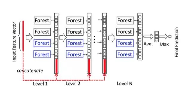
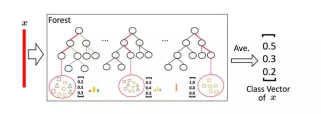
Because the decision tree is actually dividing the subspace in the feature space and labeling each subspace (the classification problem is a category and the regression problem is a target value), a test sample is given, and each tree will be based on the location of the sample. The category ratio of the training samples in the subspace generates a category probability distribution, and then averages the types of all trees in the forest to output the ratio of the entire forest to each type. For example, as shown in the figure below, this is a simplified forest based on the three classification problem of Fig. 1. Each sample will find a path in each tree to find its corresponding leaf node, and the training data in this leaf node is also the same. It is likely that there are different categories. We can statistically obtain the proportions of various types for different categories, and then average the proportions of all trees to generate the probability distribution of the entire forest.

Multi-granular scanning

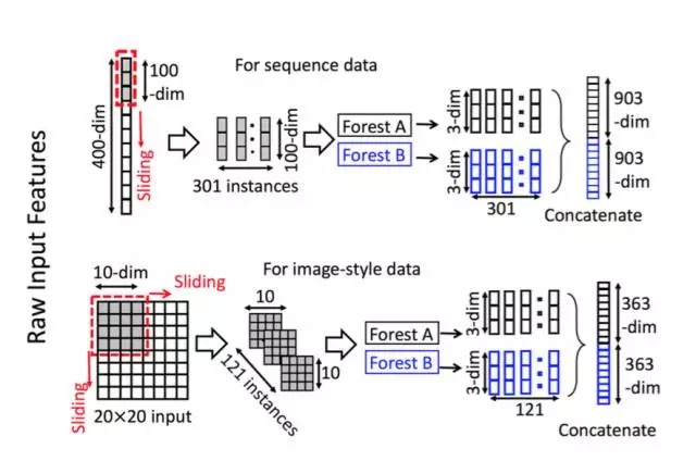
Multi-granularity scanning actually refers to a sliding window similar to CNN. For example, we now have a 400-dimensional sample input, and now set the sampling window to 100-dimensional, then we can obtain 301 sub-samples by stepwise sampling ( Therefore, the default sampling step size is 1, so the number of subsamples obtained is (400-100) / 1 + 1). If the input is a 20 * 20 picture, using a 10 * 10 sampling window, 121 subsamples can be obtained ((20-10) / 1 + 1 = 11 for each row and column, 11 * 11 = 121). Therefore, the entire multi-granularity scanning process is: first input a complete P-dimensional sample, and then slide sampling through a sampling window of length k to obtain S = (P-K) / 1 + 1 k-dimensional feature sub-sample vectors Then, each sub-sample is used for the training of completely random forest and ordinary random forest and a probability vector of length C is obtained in each forest, so that each forest will generate a characterization vector of length S * C (that is, after random Forest transformation and stitching probability vector), and finally the results of F forests in each layer are stitched together to get the output of this layer.

Algorithm implementation

In view of this, on Github, someone has implemented the algorithm code. Here we provide a code implementation method based on python3. Choose to use scikit to learn the grammar for ease of use. Here's how to use it.

The source code of GCForest.py is as follows. First you need to import this module into the root directory and name it GCForest.py. Of course, it is best to clone it from github.

gcForest in Python

Status : under development

gcForest is an algorithm suggested in Zhou and Feng 2017. It uses a multi-grain scanning approach for data slicing and a cascade structure of multiple random forests layers (see paper for details).

gcForest has been first developed as a Classifier and designed such that the multi-grain scanning module and the cascade structure can be used separately. During development I’ve paid special attention to write the code in the way that future parallelization should be pretty straightforward to implement.

Prerequisites

The present code has been developed under python3.x. You will need to have the following installed on your computer to make it work :

Python 3.x
Numpy >= 1.12.0
Scikit-learn >= 0.18.1
jupyter >= 1.0.0 (only useful to run the tuto notebook)

You can install all of them using pip install :
$ pip3 install requirements.txt

Using gcForest

The syntax uses the scikit learn style with a .fit() function to train the algorithm and a .predict() function to predict new values class. You can find two examples in the jupyter notebook included in the repository.








from GCForest import *








gcf = gcForest( **kwargs )








gcf.fit(X_train, y_train)








gcf.predict(X_test)

Notes

I wrote the code from scratch in two days and even though I have tested it on several cases I cannot certify that it is a 100% bug free obviously. Feel free to test it and send me your feedback about any improvement and/or modification!

Known Issues

Memory comsuption when slicing data There is now a short naive calculation illustrating the issue in the notebook. So far the input data slicing is done all in a single step to train the Random Forest for the Multi-Grain Scanning. The problem is that it might requires a lot of memory depending on the size of the data set and the number of slices asked resulting in memory crashes (at least on my Intel Core 2 Duo).

I have recently improved the memory usage (from version 0.1.4) when slicing the data but will keep looking at ways to optimize the code.

OOB score error During the Random Forests training the Out-Of-Bag (OOB) technique is used for the prediction probabilities. It was found that this technique can sometimes raises an error when one or several samples is/are used for all trees training.
A potential solution consists in using cross validation instead of OOB score although it slows down the training. Anyway, simply increasing the number of trees and re-running the training (and crossing fingers) is often enough.

Built With

PyCharm community edition
memory_profiler libra

License

This project is licensed under the MIT License (see LICENSE for details)

Early Results

(will be updated as new results come out)

Scikit-learn handwritten digits classification :
training time ~ 5min
accuracy ~ 98%

Part of the code:








import itertools








import numpy as np








from sklearn.ensemble import RandomForestClassifier








from sklearn.model_selection import train_test_split








from sklearn.metrics import accuracy_score

















__author__ = "Pierre-Yves Lablanche"








__email__ = "plablanche@aims.ac.za"








__license__ = "MIT"








__version__ = "0.1.3"








__status__ = "Development"

















# noinspection PyUnboundLocalVariable








class gcForest(object):








def __init__(self, shape_1X=None, n_mgsRFtree=30, window=None, stride=1,








                 cascade_test_size=0.2, n_cascadeRF=2, n_cascadeRFtree=101, cascade_layer=np.inf,








                 min_samples_mgs=0.1, min_samples_cascade=0.05, tolerance=0.0, n_jobs=1):








""" gcForest Classifier.

About scale

The main technical problem in the current implementation of gcForest is the memory usage when inputting data. Real calculations actually give you an idea of the number and size of objects that the algorithm will process.

Calculate a class C [l, L] size N-dimensional problem. The initial scale is:

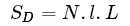
Slicing Step

If my window is of size [wl,wL] and the chosen stride are [sl,sL] then the number of slices per sample is :

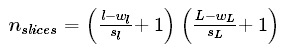
Obviously the size of slice is [wl,wL]hence the total size of the sliced data set is :

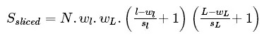
This is when the memory consumption is its peak maximum.

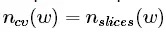
Class Vector after Multi-Grain Scanning

Now all slices are fed to the random forest to generate class vectors. The number of class vector per random forest per window per sample is simply equal to the number of slices given to the random forest

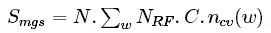
Hence, if we have Nrfrandom forest per window the size of a class vector is (recall we have N samples and C classes):

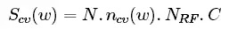
And finally the total size of the Multi-Grain Scanning output will be:

This short calculation is just meant to give you an idea of the data processing during the Multi-Grain Scanning phase. The actual memory consumption depends on the format given (aka float, int, double, etc.) and it might be worth looking at it carefully when dealing with large datasets.

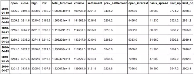
Predicting the ups and downs of each K-line

After obtaining the transaction data of each K-line, use open, close, high, low, volume, ema, macd, linreg, momentum, rsi, var, cycle, atr as the characteristic indicators, and the next K-line change as the forecast indicator








#获取当前时间








from datetime import datetime








now = datetime.now()








startDate = '2010-4-16'








endDate = now








#获取沪深300股指期货数据，频率为1分钟








df=get_price('IF88', start_date=startDate, end_date=endDate,\








frequency='1d', fields=None, country='cn')

















open = df['open'].values








close = df['close'].values








volume = df['volume'].values








high = df['high'].values








low = df['low'].values








import talib as ta








import pandas as pd








import numpy as np








from sklearn import preprocessing








ema = ta.EMA(close, timeperiod=30).tolist()








macd = ta.MACD(close, fastperiod=12, slowperiod=26, signalperiod = 9)[0].tolist()








momentum = ta.MOM(close, timeperiod=10).tolist()








rsi = ta.RSI(close, timeperiod=14).tolist()








linreg = ta.LINEARREG(close, timeperiod=14).tolist()








var = ta.VAR(close, timeperiod=5, nbdev=1).tolist()#获取当前的收盘价的希尔伯特变换








cycle = ta.HT_DCPERIOD(close).tolist()#获取平均真实波动范围指标ATR,时间段为14








atr = ta.ATR(high, low, close, timeperiod=14).tolist()#把每根k线的指标放入数组X中，并转置








X = np.array([open,close,high,low,volume,ema, macd, linreg, momentum, rsi, var, cycle, atr]).T#输出可知数组X包含了ema, macd, linreg等13个指标数值








X[2]

array ([3215., 3267.2, 3281.2, 3208., 114531.,
at, at, at, at, at, at,
at])








y=[]








c=close[0]








#用i遍历整个数据集








for i in range(1, len(X)):    








#如果高点突破参考线的1.0015倍，即上涨








if (close[i]>close[i-1]):        








#把参考点加到列表basicLine里，并且新参考点变为原来的1.0015倍，








y.append(1)        








elif (close[i]<close[i-1]): 








y.append(0)         








elif (close[i]==close[i-1]): 








y.append(2)        








#添加最后一个数据的标签为1








y.append(1)

















#把y转化为ndarray数组








y=np.array(y)








#输出验证标签集是否准确








print(len(y))








for i in range(1, 10):








print(close[i],y[i],i)

1663
3214.6 1 1
3267.2 0 2
3236.2 0 3
3221.2 0 4
3219.6 0 5
3138.8 0 6
3129.0 0 7
3083.8 1 8
3107.0 0 9








#把数据集分解成随机的训练和测试子集， 参数test_size表示测试集所占比例








X_tr, X_te, y_tr, y_te = train_test_split(X, y, test_size=0.33)








#输出可知测试特征集为维度是50*4的数组ndarray








X_te.shape

(549, 13) The
algorithm is first called and trained. The parameter shape_1X here refers to the dimension of a sample.
I also input the dimensions into the machine as image features. Obviously, it is not very relevant to the iris dataset, but still needs to be defined. The
0.1.3 version can input integers as shape_1X parameters.

gcForest parameter description

shape_1X:
the shape of a single sample element [n_lines, n_cols]. Required when calling mg_scanning! For sequence data, a single int can be given.

n_mgsRFtree: The
number of trees in the random forest during the multi-granularity scan.

window: int (default = None)
List of window sizes used during multi-granularity scanning. If None, no sectioning is performed.

stride: int (default = 1)
Step to use when slicing data.

cascade_test_size: float or int (default = 0.2)
fraction or absolute number of cascade training set splits.

n_cascadeRF: int (default = 2)
the number of random forests in the cascade layer. For each pseudo-random forest, a complete random forest is created, so the total number of random forests in a layer will be 2 * n_cascadeRF.

n_cascadeRFtree: int (default = 101) The
number of trees in a single random forest in the cascade layer.

min_samples_mgs:
The minimum number of samples to perform a split in a float or int (default = 0.1) node during multi-granularity scan random forest training. If int number_of_samples = int. If float, min_samples represents the score of the initial n_samples to be considered.

min_samples_cascade:
The minimum number of samples to perform splitting in a float or int (default = 0.1) node during cascade random forest training. If int number_of_samples = int. If float, min_samples represents the score of the initial n_samples to be considered.

cascade_layer:
the maximum number of cascade levels allowed by int (default = np.inf) . Useful for limiting cascading structures.

tolerance:
The accuracy of float (default = 0.0) cascade growth is poor. The performance of the entire cascade will be estimated on the validation set. If there is no significant performance gain, the training process will terminate

n_jobs: int (default = 1) The
number of parallel running jobs that any random forest fits and predicts. If -1, the number of jobs is set to the number of cores.








#shape_1X样本维度，window为多粒度扫描（Multi-Grained Scanning）算法中滑动窗口大小，\








#用于扫描原始数据，tolerance为级联生长的精度差,整个级联的性能将在验证集上进行估计，\








#如果没有显着的性能增益，训练过程将终止#gcf = gcForest(shape_1X=4, window=2, tolerance=0.0)








#gcf = gcForest(shape_1X=[13,13], window=2, tolerance=0.0)

















gcf = gcForest(shape_1X=13, n_mgsRFtree=100, window=6, stride=2,








cascade_test_size=0.2, n_cascadeRF=4, n_cascadeRFtree=101, cascade_layer=np.inf,








min_samples_mgs=0.1, min_samples_cascade=0.1, tolerance=0.0, n_jobs=1)








gcf.fit(X_tr, y_tr)

Slicing Sequence…
Training MGS Random Forests…
Adding/Training Layer, n_layer=1
Layer validation accuracy = 0.5577889447236181
Adding/Training Layer, n_layer=2
Layer validation accuracy = 0.521608040201005








#shape_1X样本维度，window为多粒度扫描（Multi-Grained Scanning）算法中滑动窗口大小，\








#用于扫描原始数据，tolerance为级联生长的精度差,整个级联的性能将在验证集上进行估计，\








#如果没有显着的性能增益，训练过程将终止#gcf = gcForest(shape_1X=4, window=2, tolerance=0.0)








#gcf = gcForest(shape_1X=[13,13], window=2, tolerance=0.0)

















gcf = gcForest(shape_1X=[1,13], window=[1,6],)








gcf.fit(X_tr, y_tr)

Slicing Sequence…
Training MGS Random Forests…
Slicing Sequence…
Training MGS Random Forests…
Adding/Training Layer, n_layer=1
Layer validation accuracy = 0.5964125560538116
Adding/Training Layer, n_layer=2
Layer validation accuracy = 0.5695067264573991

The parameters are changed to shape_1X = [1,13], window = [1,6], and the training set reaches 0.59, which is not ideal. Here we are just introducing bricks and stones. Adjusting parameters requires the guidance of a great god.

Now checking the prediction for the test set
:








pred_X = gcf.predict(X_te)








print(len(pred_X))








print(len(y_te))








print(pred_X)

Slicing Sequence…
Slicing Sequence…
549
549
[1 1 0 0 0 0 0 0 0 0 1 0 0 0 1 0 1 1 0 1 0 1 0 1 0 0 0 0 0 0 1 1 1 0 0 1 0等








#最近预测








for i in range(1,len(pred_X)):








print(y_te[-i],pred_X[-i],-i)

0 1 -1
0 0 -2
1 0 -3
1 0 -4
0 1 -5
etc.








# 保存每一天预测的结果，如果某天预测对了，保存1，如果某天预测错了，保存-1








result_list = []








# 检查预测是否成功

















def checkPredict(i):








if pred_X[i] == y_te[i]:








result_list.append(1)    








else:








result_list.append(0)








#画出最近第k+1个长度为j的时间段准确率








k=0j








=len(y_te)








#j=100








for i in range(len(y_te)-j*(k+1), len(y_te)-j*k):








checkPredict(i)    








#print(y_pred[i])








#return result_list








print(len(y_te) ) 








print(len(result_list) )

















import matplotlib.pyplot as plt








#将准确率曲线画出来








x = range(0, len(result_list))








y = []








#z=[]








for i in range(0, len(result_list)):    








#y.append((1 + float(sum(result_list[:i])) / (i+1)) / 2)








y.append( float(sum(result_list[:i])) / (i+1))








print('最近',j,'次准确率',y[-1])








print(x, y)








line, = plt.plot(x, y)








plt.show

549
549
most recent 549 accuracy 0.5300546448087432
range (0, 549) [0.0, 0.0, 0.3333333333333333, 0.25 etc.








#评估准确率








# evaluating accuracy








accuracy = accuracy_score(y_true=y_te, y_pred=pred_X)








print('gcForest accuracy : {}'.format(accuracy))

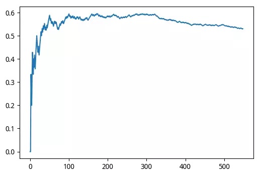
gcForest accuracy: 0.5300546448087432 The
prediction result is average, but it is still valid.
Predicting the ups and downs is not so reliable, but the recognition of handwritten numbers is still quite good.

Only the results are posted below:








# loading the data

















digits = load_digits()








X = digits.data








y = digits.target








X_tr, X_te, y_tr, y_te = train_test_split(X, y, test_size=0.4)








gcf = gcForest(shape_1X=[7,8], window=[4,6], tolerance=0.0, min_samples_mgs=10, min_samples_cascade=7)








#gcf = gcForest(shape_1X=13, window=13, tolerance=0.0, min_samples_mgs=10, min_samples_cascade=7)








gcf.fit(X_tr, y_tr)

Slicing Images…
Training MGS Random Forests…
Slicing Images…
Training MGS Random Forests…
Adding/Training Layer, n_layer=1
Layer validation accuracy = 0.9814814814814815
Adding/Training Layer, n_layer=2
Layer validation accuracy = 0.9814814814814815








# evaluating accuracy








accuracy = accuracy_score(y_true=y_te, y_pred=pred_X)








print('gcForest accuracy : {}'.format(accuracy))

gcForest accuracy: 0.980528511821975 is
great, simple parameters can make the accuracy of handwritten digit recognition as high as 98%

Take advantage of multi-granular scanning and cascading forests separately

Since the multi-granularity scanning and cascading forest modules are quite independent, they can be used separately.

If given the target "y", the code will automatically use it for training, otherwise it will call the last trained random forest to split the data.








gcf = gcForest(shape_1X=[8,8], window=5, min_samples_mgs=10, min_samples_cascade=7)








X_tr_mgs = gcf.mg_scanning(X_tr, y_tr)

Slicing Images…
Training MGS Random Forests…
It is now possible to use the mg_scanning output as input for cascade forests using different parameters. Note that the cascade forest module does not directly return predictions but probability predictions from each Random Forest in the last layer of the cascade. Hence the need to first take the mean of the output and then find the max.








gcf = gcForest(tolerance=0.0, min_samples_mgs=10, min_samples_cascade=7)








_ = gcf.cascade_forest(X_tr_mgs, y_tr)

Adding/Training Layer, n_layer=1
Layer validation accuracy = 0.9722222222222222
Adding/Training Layer, n_layer=2
Layer validation accuracy = 0.9907407407407407
Adding/Training Layer, n_layer=3
Layer validation accuracy = 0.9814814814814815








import numpy as np








pred_proba = gcf.cascade_forest(X_te_mgs)








tmp = np.mean(pred_proba, axis=0)








preds = np.argmax(tmp, axis=1)








accuracy_score(y_true=y_te, y_pred=preds)








gcf = gcForest(tolerance=0.0, min_samples_mgs=20, min_samples_cascade=10)








_ = gcf.cascade_forest(X_tr_mgs, y_tr)








pred_proba = gcf.cascade_forest(X_te_mgs)








tmp = np.mean(pred_proba, axis=0)








preds = np.argmax(tmp, axis=1)








accuracy_score(y_true=y_te, y_pred=preds)

0.97774687065368571
Adding/Training Layer, n_layer=1
Layer validation accuracy = 0.9629629629629629
Adding/Training Layer, n_layer=2
Layer validation accuracy = 0.9675925925925926
Adding/Training Layer, n_layer=3
Layer validation accuracy = 0.9722222222222222
Adding/Training Layer, n_layer=4
Layer validation accuracy = 0.9722222222222222
0.97218358831710705

Skipping mg_scanning

It is also possible to directly use the cascade forest and skip the multi grain scanning step.








gcf = gcForest(tolerance=0.0, min_samples_cascade=20)








_ = gcf.cascade_forest(X_tr, y_tr)








pred_proba = gcf.cascade_forest(X_te)








tmp = np.mean(pred_proba, axis=0)








preds = np.argmax(tmp, axis=1)








accuracy_score(y_true=y_te, y_pred=preds)

Adding/Training Layer, n_layer=1
Layer validation accuracy = 0.9583333333333334
Adding/Training Layer, n_layer=2
Layer validation accuracy = 0.9675925925925926
Adding/Training Layer, n_layer=3
Layer validation accuracy = 0.9583333333333334
0.94297635605006958

চাউ ঝিহুয়ার নিবন্ধের জন্য, কেউ অনলাইনে খুব বিস্তারিত ব্যাখ্যা দিয়েছেন। আমরা সংক্ষিপ্তভাবে কাগজটি বর্ণনা করার পরে, আমরা কৌশলটি দিয়ে শুরু করি।

gcForest (মাল্টি-গ্রেইন্ডেড ক্যাসকেড অরণ্য) অধ্যাপক ঝো ঝিহুয়া প্রস্তাবিত একটি নতুন সিদ্ধান্ত গাছ সংহতকরণ পদ্ধতি। এই পদ্ধতিটি একটি গভীর অরণ্য সংগ্রহের পদ্ধতি তৈরি করে এবং জিসিফোরস্টের জন্য শিখতে একটি ক্যাসকেড কাঠামো ব্যবহার করে। জিসিফোরস্ট মডেল প্রশিক্ষণকে দুটি পর্যায়ে বিভক্ত করে: মাল্টি-গ্রেইন্ডেড স্ক্যানিং এবং ক্যাসকেড ফরেস্ট। মাল্টি-গ্রেইন্ড স্ক্যানিং বৈশিষ্ট্য উত্পন্ন করে এবং ক্যাসকেড ফরেস্ট পূর্বাভাসের ফলাফলগুলি পেতে একাধিক বনকে ক্যাসকেড করে।

এর প্রতিনিধিত্বমূলক শিক্ষার ক্ষমতা উচ্চ-মাত্রিক ইনপুট ডেটার মাল্টি-গ্রানুলারিটি স্ক্যানিং দ্বারা বাড়ানো যেতে পারে। সিরিজের স্তরগুলির সংখ্যাটিও অভিযোজিতভাবে নির্ধারণ করা যেতে পারে যাতে মডেল জটিলতাটি কাস্টম হাইপারপ্যারামিটার হওয়ার প্রয়োজন হয় না, তবে একটি পরামিতি যা ডেটা পরিস্থিতি অনুসারে স্বয়ংক্রিয়ভাবে সেট হয়। এটি লক্ষণীয় যে gcForest এর ডিএনএন এর চেয়ে কম হাইপারপ্যারামিটার থাকবে। ভাল জিনিস হ'ল gcForest পরামিতিগুলির জন্য খুব মজবুত। এমনকি ডিফল্ট প্যারামিটারগুলির সাথেও, আপনি দুর্দান্ত ফলাফল পেতে পারেন।

ক্যাসকেড ফরেস্ট

ছবির বর্ণনা

কারণ সিদ্ধান্ত গাছটি প্রকৃতপক্ষে বৈশিষ্ট্যের জায়গার মধ্যে উপ-স্থানটিকে বিভাজন করছে এবং প্রতিটি উপস্থানে লেবেল দিচ্ছে (শ্রেণিবদ্ধকরণ সমস্যাটি একটি বিভাগ এবং রেগ্রেশন সমস্যা একটি লক্ষ্য মান), একটি পরীক্ষার নমুনা দেওয়া হয় এবং প্রতিটি গাছের অবস্থানের ভিত্তিতে তৈরি করা হবে নমুনা. উপ-স্থানের প্রশিক্ষণের নমুনাগুলির বিভাগ অনুপাত একটি বিভাগ সম্ভাবনা বন্টন তৈরি করে এবং তারপরে বনের সমস্ত গাছের প্রকারভেদকে পুরো বনের অনুপাত প্রতিটি ধরণের আউটপুট করতে দেয় verages উদাহরণস্বরূপ, নীচের চিত্রে যেমন দেখানো হয়েছে, ডুমুরের তিনটি শ্রেণিবিন্যাস সমস্যার উপর ভিত্তি করে এটি একটি সরল বনভূমি Each. প্রতিটি নমুনা প্রতিটি গাছের সাথে সম্পর্কিত পাতার নোড এবং এই পাতার নোডে প্রশিক্ষণের ডেটা সন্ধান করবে একই। এটি সম্ভবত বিভিন্ন বিভাগ রয়েছে বলে মনে হয়। আমরা পরিসংখ্যানগতভাবে বিভিন্ন বিভাগের জন্য বিভিন্ন ধরণের অনুপাত পেতে পারি এবং তারপরে পুরো বনের সম্ভাব্যতা বন্টন তৈরি করতে সমস্ত গাছের অনুপাতকে গড়ে তুলতে পারি।

ছবির বর্ণনা

মাল্টি-দানাদার স্ক্যানিং

ছবির বর্ণনা

মাল্টি-গ্রানুলারিটি স্ক্যানিং আসলে সিএনএন এর অনুরূপ একটি স্লাইডিং উইন্ডোকে বোঝায়। উদাহরণস্বরূপ, এখন আমাদের কাছে 400-মাত্রিক নমুনা ইনপুট রয়েছে এবং এখন স্যাম্পলিং উইন্ডোটি 100-মাত্রিক হিসাবে সেট করা হয়েছে, তারপরে আমরা ধাপে ধাপে নমুনা দিয়ে 301 উপ-নমুনা পেতে পারি (অতএব, ডিফল্ট নমুনা ধাপের আকার 1, সুতরাং সংখ্যাটি প্রাপ্ত নমুনাগুলি হ'ল (400-100) / 1 + 1)। যদি ইনপুটটি 20 * 20 টি চিত্র হয়, 10 * 10 স্যাম্পলিং উইন্ডো ব্যবহার করে, 121 টি নমুনা পাওয়া যাবে ((20-10) / 1 + 1 = 11 প্রতিটি সারি এবং কলামের জন্য, 11 * 11 = 121)। সুতরাং, সম্পূর্ণ মাল্টি-গ্রানুলারিটি স্ক্যানিং প্রক্রিয়াটি হ'ল: প্রথমে সম্পূর্ণ পি-ডাইমেনশনাল নমুনা ইনপুট করুন এবং তারপরে এস = (পিকে) / 1 + 1 কে-মাত্রিক বৈশিষ্ট্য উপ-নমুনা ভেক্টরগুলি পেতে দৈর্ঘ্যের কে এর একটি নমুনা উইন্ডো দিয়ে স্যাম্পলিং স্লাইড করুন তারপরে, প্রতিটি উপ-নমুনা সম্পূর্ণরূপে এলোমেলো বন এবং সাধারণ এলোমেলো বন প্রশিক্ষণের জন্য ব্যবহৃত হয় এবং প্রতিটি বনাঞ্চলে দৈর্ঘ্যের সি এর সম্ভাব্যতা ভেক্টর প্রাপ্ত হয়, যাতে প্রতিটি অরণ্য দৈর্ঘ্যের এস * সি এর বৈশিষ্ট্যযুক্ত ভেক্টর তৈরি করে (যা, এলোমেলোভাবে বন রূপান্তর এবং সম্ভাবনার ভেক্টর সেলাইয়ের পরে) এবং শেষ পর্যন্ত প্রতিটি স্তরের এফ বনাঞ্চলের ফলাফলগুলি এই স্তরের আউটপুট পেতে একসাথে সেলাই করা হয়।

অ্যালগরিদম বাস্তবায়ন

এর পরিপ্রেক্ষিতে, গিথুব-এ, কেউ আলগোরিদিম কোডটি প্রয়োগ করেছেন। এখানে আমরা পাইথন 3 এর উপর ভিত্তি করে একটি কোড বাস্তবায়ন পদ্ধতি সরবরাহ করি। ব্যবহারের সহজতার জন্য ব্যাকরণ শিখতে বিজ্ঞান ব্যবহার করতে বেছে নিন। এটি কীভাবে ব্যবহার করবেন তা এখানে।

GCForest.py এর উত্স কোডটি নিম্নরূপ। প্রথমে আপনাকে এই মডিউলটি মূল ডিরেক্টরিতে আমদানি করতে হবে এবং এর নাম দিতে হবে জিসিফোরস্ট.পি py অবশ্যই, এটি গিথুব থেকে ক্লোন করা ভাল।

পাইথনে gcForest

স্থিতি: বিকাশের অধীনে

জিসিফোরেস্টটি ঝো এবং ফেং 2017 এ প্রস্তাবিত একটি অ্যালগরিদম It এটি ডেটা স্লাইস করার জন্য একটি বহু-শস্য স্ক্যানিং পদ্ধতি এবং একাধিক এলোমেলো বন স্তরগুলির একটি ক্যাসকেড কাঠামো ব্যবহার করে (বিশদ জন্য কাগজ দেখুন)।

gcForest প্রথমে ক্লাসিফায়ার হিসাবে বিকাশ করা হয়েছে এবং এমনভাবে ডিজাইন করা হয়েছে যে মাল্টি-শস্য স্ক্যানিং মডিউল এবং ক্যাসকেড কাঠামো পৃথকভাবে ব্যবহার করা যেতে পারে। উন্নয়নের সময় আমি কোডটি লেখার জন্য বিশেষ মনোযোগ দিয়েছি যাতে ভবিষ্যতের সমান্তরালাকে কার্যকর করার জন্য বেশ সহজবোধ্য হওয়া উচিত।

পূর্বশর্ত

বর্তমান কোডটি পাইথন 3.x এর অধীনে তৈরি করা হয়েছে। এটিকে কাজ করতে আপনার কম্পিউটারে নিম্নলিখিতটি ইনস্টল করা প্রয়োজন:

পাইথন 3.x

নম্পি> = 1.12.0

সাইকিট-শিখুন> = 0.18.1

jupyter> = 1.0.0 (টুটো নোটবুক চালাতে কেবল কার্যকর)

আপনি পাইপ ইনস্টল ব্যবহার করে সেগুলি সবগুলি ইনস্টল করতে পারেন:

$ পাইপ 3 ইনস্টল করা প্রয়োজনীয়তা.টিএসটিএসটি

GcForest ব্যবহার করে

সিনট্যাক্সটি অ্যালগরিদমকে প্রশিক্ষণের জন্য একটি। ফিট () ফাংশন সহ একটি স্কিটিট লার্ন স্টাইল এবং নতুন মান শ্রেণীর পূর্বাভাস দেওয়ার জন্য একটি প্রেডিক্ট () ফাংশন ব্যবহার করে। সংগ্রহস্থলের অন্তর্ভুক্ত জুপিটার নোটবুকে আপনি দুটি উদাহরণ পেতে পারেন।

from GCForest import *
gcf = gcForest( **kwargs )
gcf.fit(X_train, y_train)
gcf.predict(X_test)

মন্তব্য

আমি কোডটি স্ক্র্যাচ থেকে দুদিনের মধ্যে লিখেছি এবং যদিও আমি বেশ কয়েকটি ক্ষেত্রে এটি পরীক্ষা করে দেখেছি তবে আমি প্রমাণ করতে পারি না যে এটি অবশ্যই 100% বাগ বিনামূল্যে। এটি নির্দ্বিধায় নিখরচায় এবং কোনও উন্নতি এবং / বা পরিবর্তন সম্পর্কে আপনার প্রতিক্রিয়া আমাকে পাঠান!

জ্ঞাত সমস্যা

ডেটা টুকরা করার সময় স্মৃতি সংমিশ্রণটি নোটবুকটিতে সমস্যাটি চিত্রিত করার জন্য একটি ছোট্ট নির্লজ্জ গণনা রয়েছে। মাল্টি-গ্রেইন স্ক্যানিংয়ের জন্য র্যান্ডম ফরেস্টকে প্রশিক্ষণের জন্য এখনও অবধি ইনপুট ডেটা স্লাইসিং একক পদক্ষেপে সম্পন্ন হয়েছে। সমস্যাটি হ'ল এতে ডেটা সেটের আকার এবং মেমরি ক্র্যাশ হওয়ার ফলে জিজ্ঞাসা করা টুকরোগুলির সংখ্যার উপর নির্ভর করে (কমপক্ষে আমার ইন্টেল কোর 2 ডুও) এর জন্য প্রচুর মেমরির প্রয়োজন হতে পারে।

ডেটা স্লাইস করার সময় আমি সম্প্রতি মেমরির ব্যবহারের উন্নতি করেছি (০.০.৪ সংস্করণ থেকে) তবে কোডটি অনুকূলিত করার উপায়গুলি দেখব।

OOB স্কোর ত্রুটি র্যান্ডম অরণ্য প্রশিক্ষণের সময় ভবিষ্যদ্বাণী সম্ভাবনার জন্য আউট-অফ-ব্যাগ (OOB) কৌশল ব্যবহার করা হয়। এটি পাওয়া গিয়েছিল যে সমস্ত গাছ প্রশিক্ষণের জন্য যখন এক বা একাধিক নমুনা ব্যবহৃত হয় / ব্যবহৃত হয় তখন এই কৌশলটি কখনও কখনও ত্রুটি তৈরি করতে পারে।

একটি সম্ভাব্য সমাধান ওওবি স্কোরের পরিবর্তে ক্রস বৈধকরণ ব্যবহার করে তবে এটি প্রশিক্ষণটি ধীর করে দেয়। যাইহোক, কেবলমাত্র গাছের সংখ্যা বাড়ানো এবং প্রশিক্ষণটি পুনরায় চালানো (এবং আঙ্গুলগুলি অতিক্রম করা) প্রায়শই যথেষ্ট।

দিয়ে নির্মিত

পাইচর্ম সম্প্রদায় সংস্করণ

মেমরি_ প্রোফেলার লাইব্রেরি

লাইসেন্স

এই প্রকল্পটি এমআইটি লাইসেন্সের আওতায় লাইসেন্সযুক্ত (বিশদ জন্য লাইসেন্স দেখুন)

প্রাথমিক ফলাফল

(নতুন ফলাফল প্রকাশের সাথে সাথে আপডেট করা হবে)

সাইকিট-শিখুন হস্তাক্ষর অঙ্কের শ্রেণিবিন্যাস:

প্রশিক্ষণের সময় 5 মিনিট

নির্ভুলতা ~ 98%

Part of the code:








import itertools








import numpy as np








from sklearn.ensemble import RandomForestClassifier








from sklearn.model_selection import train_test_split








from sklearn.metrics import accuracy_score

















__author__ = "Pierre-Yves Lablanche"








__email__ = "plablanche@aims.ac.za"








__license__ = "MIT"








__version__ = "0.1.3"








__status__ = "Development"

















# noinspection PyUnboundLocalVariable








class gcForest(object):








def __init__(self, shape_1X=None, n_mgsRFtree=30, window=None, stride=1,








                 cascade_test_size=0.2, n_cascadeRF=2, n_cascadeRFtree=101, cascade_layer=np.inf,








                 min_samples_mgs=0.1, min_samples_cascade=0.05, tolerance=0.0, n_jobs=1):








""" gcForest Classifier.

প্রায় স্কেল

জিসিফোরেস্টের বর্তমান প্রয়োগে মূল প্রযুক্তিগত সমস্যা হ'ল ডেটা ইনপুট করার সময় মেমরির ব্যবহার। আসল গণনাগুলি আসলে আপনাকে অ্যালগোরিদম প্রক্রিয়া করবে এমন বস্তুর সংখ্যা এবং আকার সম্পর্কে ধারণা দেয়।

একটি শ্রেণি সি [l, L] আকারের N- মাত্রিক সমস্যা গণনা করুন Calc প্রাথমিক স্কেলটি হ'ল:

কাটা পদক্ষেপ

যদি আমার উইন্ডোটি আকারের হয় [wl, wL] এবং নির্বাচিত স্ট্রাইড [sl, sL] হয় তবে নমুনা অনুসারে স্লাইসের সংখ্যাটি হ'ল:

মাল্টি-গ্রেইন স্ক্যানের পরে ক্লাস ভেক্টর

ক্লাস ভেক্টরগুলি তৈরি করতে এখন সমস্ত টুকরোগুলি এলোমেলো বনগুলিতে খাওয়ানো হয়। নমুনা প্রতি উইন্ডোতে এলোমেলো বন প্রতি বর্গ ভেক্টরের সংখ্যা কেবল এলোমেলো বনগুলিতে প্রদত্ত টুকরো সংখ্যার সমান

Mohammad Mostofa Zaman

gcForest algorithm