পর্ব 1
Let's start with some biology
মস্তিষ্কের স্নায়ু কোষকে নিউরন বলে। মানুষের মস্তিষ্কে পাওয়ার (1010) নিউরনগুলির একটি আনুমানিক 1010 রয়েছে। প্রতিটি নিউরন কয়েক হাজার অন্যান্য নিউরনের সাথে যোগাযোগ করতে পারে। নিউরন হ'ল একক যা মস্তিষ্ক তথ্য প্রক্রিয়াকরণের জন্য ব্যবহার করে
So what does a neuron look like
নিউরনে একটি সেল বডি থাকে, যার থেকে বিভিন্ন এক্সটেনশন থাকে। এর বেশিরভাগই ডেনড্রাইট নামে পরিচিত শাখা branches অ্যাক্সন নামে আরও একটি দীর্ঘ প্রক্রিয়া রয়েছে (সম্ভবত ব্রাঞ্চিংও)। ড্যাশড লাইনটি অ্যাক্সন টিলা দেখায়, যেখানে সংকেতগুলির সংক্রমণ শুরু হয় নিম্নলিখিত চিত্রটি এটি চিত্রিত করে।
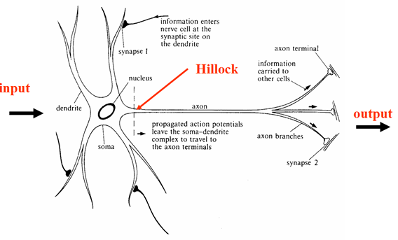
Figure 1 Neuron
নিউরনের সীমানা কোষের ঝিল্লি হিসাবে পরিচিত। ঝিল্লির অভ্যন্তর এবং বাইরের মধ্যে ভোল্টেজের পার্থক্য (ঝিল্লি সম্ভাবনা) রয়েছে। যদি ইনপুটটি যথেষ্ট পরিমাণে বড় হয় তবে একটি ক্রিয়া সম্ভাবনা উত্পন্ন হয়। অ্যাকশন সম্ভাবনা (নিউরোনাল স্পাইক) এর পরে সেল বডি থেকে দূরে অ্যাক্সন থেকে নীচে ভ্রমণ করে।
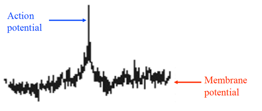
Figure 2 Neuron Spiking
Synapses
একটি নিউরনের সাথে অন্যটির মধ্যে সংযোগগুলিকে সিনাপেস বলে। তথ্য সর্বদা তার অ্যাক্সন দিয়ে নিউরনকে ছেড়ে যায় (উপরের চিত্র 1 দেখুন) এবং তারপরে একটি স্ন্যাপস জুড়ে প্রাপ্ত নিউরনে স্থানান্তরিত হয়।
Neuron Firing
ইনপুট কিছু প্রান্তিকের চেয়ে বড় হলে কেবল নিউরনগুলিতে আগুন লাগে। তবে এটি লক্ষ করা উচিত যে উদ্দীপনা বৃদ্ধি পাওয়ার সাথে সাথে গুলি ছোঁড়া বড় হয় না, এটি সমস্ত কিছুর কোনও ব্যবস্থা নয়।
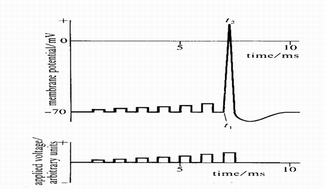
Figure 3 Neuron Firing
স্পাইকস (সিগন্যাল) গুরুত্বপূর্ণ, যেহেতু অন্যান্য নিউরন সেগুলি গ্রহণ করে। নিউরন স্পাইকের সাথে যোগাযোগ করে। প্রেরিত তথ্য স্পাইক দ্বারা কোড করা হয়।
The input to a Neuron
সিনাপেস উত্তেজক বা বাধা হতে পারে। উত্তেজনাপূর্ণ সিন্যাপে স্পাইকগুলি (সংকেতগুলি) উপস্থিতি গ্রহণকারী নিউরনকে আগুনের কারণ হতে থাকে। ইনহিবিটরি সিনপাসে উপস্থিত স্পাইকস (সিগন্যাল) গুলি ছোঁড়া থেকে প্রাপ্ত নিউরনকে বাধা দেয়। কোষের দেহ এবং সিনাপেসগুলি মূলত গণনা করা হয় (একটি জটিল রাসায়নিক / বৈদ্যুতিক প্রক্রিয়া দ্বারা) আগত উত্তেজনাপূর্ণ এবং বাধা ইনপুটগুলির মধ্যে (পার্থক্যগত এবং অস্থায়ী সংমিশ্রণ) পার্থক্য। যখন এই পার্থক্যটি যথেষ্ট পরিমাণে বড় হয় (নিউরনের প্রান্তিকের সাথে তুলনা করা হয়) তখন নিউরন গুলি ছোঁড়াবে। মোটামুটিভাবে বলতে গেলে, উত্তেজনাপূর্ণ স্পাইকগুলি এর সিনাপেসে দ্রুত পৌঁছায় তত দ্রুত আগুন লাগবে (একইভাবে ইনহিবিটরি স্পাইকগুলির জন্য)।
So how about artificial neural networks
মনে করুন যে প্রতিটি নিউরনে আমাদের ফায়ারিং রেট রয়েছে। এছাড়াও ধরুন যে নিউরন এম অন্যান্য নিউরনের সাথে সংযোগ স্থাপন করেছে এবং তাই এম-বহু ইনপুটগুলি "x1…… xm" পেয়েছে, আমরা এই কনফিগারেশনটির মতো দেখতে কিছুটা কল্পনা করতে পারি:
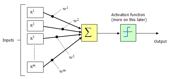
Figure 4 Artificial Neuron configuration
এই কনফিগারেশনটিকে আসলে পারসেপ্ট্রন বলা হয়। পার্সেপেট্রন (রোজেনব্ল্যাট [১৯62২]] আবিষ্কার, এটি প্রথম দিকের নিউরাল নেটওয়ার্ক মডেলগুলির মধ্যে একটি। একটি পেরসেপট্রন মডেলগুলি নিউরনের মডেলগুলি ইনপুটগুলির একটি ওজনযুক্ত সমষ্টি গ্রহণ করে এবং আউটপুট 1 প্রেরণ করে, যোগফল যদি কিছু সামঞ্জস্যযোগ্য প্রান্তিক মানের চেয়ে বেশি হয় (অন্যথায় এটি 0 প্রেরণ করে - এটিই জীববিজ্ঞানে বর্ণিত সমস্ত বা কিছুই স্পিকিং নয়, দেখুন নিউরন ফায়ারিং বিভাগটি উপরে) এটিকে অ্যাক্টিভেশন ফাংশনও বলা হয়।
চিত্র 4-এ ইনপুট (এক্স 1, এক্স 2, এক্স 3..এক্সএম) এবং সংযোগ ওজন (ডাব্লু 1, ডাব্লু 2, ডাব্লু 3 ডাব্লুএম) সাধারণত প্যাসিভ (+) এবং নেতিবাচক (-) উভয়ই আসল মান। যদি কিছু Xi এর বৈশিষ্ট্যটি পার্সেপট্রনটিকে আগুনের দিকে চালিত করে, তবে ওয়েট উইই ইতিবাচক হবে; বৈশিষ্ট্য Xi যদি পার্সেপট্রনকে বাধা দেয় তবে ওজন উইট নেতিবাচক হবে।
পার্সেপট্রন নিজেই ওজন, সামিট প্রসেসর এবং একটি অ্যাক্টিভেশন ফাংশন এবং একটি সামঞ্জস্যযোগ্য থ্রেশহোল্ড প্রসেসর (পরে এখানে পক্ষপাত বলা হয়) নিয়ে গঠিত।
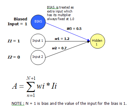
সুবিধার্থে স্বাভাবিক অনুশীলন হ'ল পক্ষপাতদুষ্ট, অন্য একটি ইনপুট হিসাবে আচরণ করা। নিম্নলিখিত চিত্রটি সংশোধিত কনফিগারেশন চিত্রিত করে।
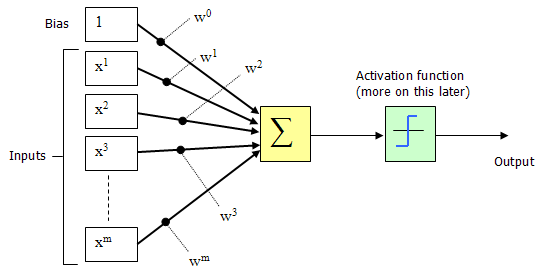
Figure 5 Artificial Neuron configuration, with bias as additinal input
পক্ষপাতদুটি তার ইনপুট নির্বিশেষে বোধ করার জন্য পার্সেপ্রেসনের প্রবণতা (আচরণের একটি নির্দিষ্ট পদ্ধতির দিকে ঝোঁক) হিসাবে বিবেচনা করা যেতে পারে। চিত্রের 5 টিতে দেখানো পার্সেপট্রন কনফিগারেশন নেটওয়ার্ক যদি ওজনযুক্ত যোগফল> 0 হয় বা আপনি যদি গণিত-ধরণের ব্যাখ্যাতে থাকেন তবে

Activation Function
The activation usually uses one of the following functions.
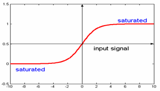
Sigmoid Function
ইনপুট যত তত শক্ত, নিউরনের আগুন দ্রুততর হবে (ফায়ারিং হার বেশি) higher সিগময়েড মাল্টি-লেয়ার নেটওয়ার্কগুলিতেও খুব দরকারী, কারণ সিগময়েড বক্ররেখা বিভিন্নকরণের জন্য অনুমতি দেয় (যা মাল্টি লেয়ার নেটওয়ার্কগুলির পিছনে প্রচার প্রশিক্ষণে প্রয়োজনীয়)।
or if your into maths type explanations

Step Function
A basic on/off type function, if 0 > x then 0, else if x >= 0 then 1

or if your into math-type explanations

Learning
A foreword on learning
পার্সেপট্রন শেখার বিষয়ে কথা বলার আগে আমরা আসল বিশ্বের উদাহরণ বিবেচনা করতে পারি:
আপনি কীভাবে একটি শিশুকে চেয়ার চিনতে শেখাবেন? আপনি তাকে উদাহরণগুলি দেখিয়ে বলছেন, "এটি একটি চেয়ার That এটি চেয়ার নয়" "যতক্ষণ না শিশু একটি চেয়ার কী তা ধারণাটি না শিখলে। এই পর্যায়ে, শিশুটি আমরা তাকে যে উদাহরণ দেখিয়েছি তার দিকে নজর দিতে এবং জিজ্ঞাসা করা হলে সঠিক উত্তর দিতে পারে, "এই বিষয়টি কি চেয়ার?"
তদুপরি, আমরা যদি শিশুটিকে নতুন কোনও বস্তু প্রদর্শন করি যা সে আগে দেখেনি, তবে আমরা তাকে প্রত্যাশা করতে পারি যে তিনি নতুন জিনিসটি চেয়ার কিনা তা সঠিকভাবে সনাক্ত করতে পারে, তবে আমরা তাকে যথেষ্ট ইতিবাচক এবং নেতিবাচক উদাহরণ দিয়েছি।
পার্সপিট্রনের পিছনে এই ধারণাটি ঠিক।
Learning in perceptrons
ওজন এবং পক্ষপাতিত্ব সংশোধন প্রক্রিয়া হয়। একটি পার্সেপট্রন তার ইনপুটটির বাইনারি ফাংশন গণনা করে। যে কোনও পার্সেপ্রেশন গণনা করতে পারে তা গণনা শিখতে পারে।
"পারসেপ্ট্রন হ'ল এমন একটি প্রোগ্রাম যা ধারণাগুলি শিখায়, অর্থাত্ এটি উপস্থাপনের জন্য বারবার" অধ্যয়ন "করে উদাহরণগুলি উপস্থাপনের জন্য সত্য (1) বা মিথ্যা (0) দিয়ে প্রতিক্রিয়া জানানো শিখতে পারে।
পারসেপ্ট্রন হ'ল একটি একক স্তর নিউরাল নেটওয়ার্ক যার ওজন এবং বায়াসগুলি সংশ্লিষ্ট ইনপুট ভেক্টরের সাথে উপস্থাপিত হলে সঠিক টার্গেট ভেক্টর উত্পাদন করতে প্রশিক্ষিত হতে পারে। ব্যবহৃত প্রশিক্ষণ কৌশলকে পার্সেপেট্রন লার্নিং রুল বলে। এই প্রশিক্ষণ ভেক্টর থেকে সাধারণীকরণ এবং এলোমেলোভাবে বিতরণ সংযোগগুলির সাথে কাজ করার দক্ষতার কারণে পার্সেপট্রন দুর্দান্ত আগ্রহ অর্জন করেছিল। পার্সেপট্রনগুলি প্যাটার্ন শ্রেণিবিন্যাসে সাধারণ সমস্যার জন্য বিশেষত উপযুক্ত ""
অধ্যাপক জিয়ানফেং ফেং, বৈজ্ঞানিক কম্পিউটিং কেন্দ্র, ইংল্যান্ডের ওয়ারউইক বিশ্ববিদ্যালয় England
The Learning Rule
পার্সেপেট্রন প্রতিটি ইনপুট ভেক্টরকে 0 বা 1 এর সাথে সম্পর্কিত টার্গেট আউটপুট দিয়ে প্রতিক্রিয়া জানাতে প্রশিক্ষিত হয় লার্নিং রুল একটি সলিউশন উপস্থিত থাকলে সীমাবদ্ধ সময়ে একটি সমাধানে রূপান্তরিত করার জন্য প্রমাণিত হয়েছে।
নিম্নোক্ত দুটি সমীকরণে শিক্ষার নিয়ম সংক্ষেপিত করা যেতে পারে:
b = b + [ T - A ]
For all inputs i:
W(i) = W(i) + [ T - A ] * P(i)
Where W is the vector of weights, P is the input vector presented to the network, T is the correct result that the neuron should have shown, A is the actual output of the neuron, and b is the bias.
Training
Vectors from a training set are presented to the network one after another.
If the network's output is correct, no change is made.
অন্যথায়, ওজন এবং বায়াসগুলি পার্সেপট্রন শিখার নিয়ম (উপরে বর্ণিত হিসাবে) ব্যবহার করে আপডেট করা হয়। ট্রেনিং সেটের প্রতিটি ইউপ (সমস্ত ইনপুট প্রশিক্ষণ ভেক্টরগুলির মধ্য দিয়ে একটি পুরো পাস বলা হয়) কোনও ত্রুটি ছাড়াই ঘটেছে, প্রশিক্ষণ সম্পূর্ণ।
এই সময়ে কোনও ইনপুট প্রশিক্ষণ ভেক্টর নেটওয়ার্কে উপস্থাপিত হতে পারে এবং এটি সঠিক আউটপুট ভেক্টরের সাথে প্রতিক্রিয়া জানাবে। যদি কোনও ভেক্টর, পি, ট্রেনিং সেটে নেটওয়ার্কে উপস্থাপন না করা হয়, তবে নেটওয়ার্কটি আগে দেখা যায়নি ইনপুট ভেক্টর পি এর কাছাকাছি ইনপুট ভেক্টরগুলির জন্য টার্গেট ভেক্টরগুলির অনুরূপ একটি আউটপুট দিয়ে প্রতিক্রিয়া দেখিয়ে সাধারণীকরণ প্রদর্শন করবে
So what can we use do with neural networks
ঠিক আছে, যদি আমরা একটি একক স্তর নিউরাল নেটওয়ার্ক ব্যবহার করতে থাকি, যে কাজগুলি অর্জন করা যায় সেগুলি মাল্টি-লেয়ার নিউরাল নেটওয়ার্কগুলি দ্বারা অর্জন করা যেতে পারে তার চেয়ে আলাদা from যেহেতু এই নিবন্ধটি মূলত একক স্তর নেটওয়ার্কগুলির সাথে ডিল করার দিকে মনোনিবেশ করা হয়েছে, আসুন সেগুলি আরও বিশদভাবে দেখি:
Single layer neural networks
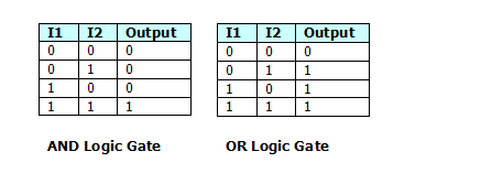
সিঙ্গল-লেয়ার নিউরাল নেটওয়ার্কস (পার্সেপেট্রন নেটওয়ার্ক) এমন একটি নেটওয়ার্ক যা যেখানে আউটপুট ইউনিট অন্যদের থেকে স্বতন্ত্র - প্রতিটি ওজন কেবল একটি আউটপুটকে প্রভাবিত করে। পার্সেপেট্রন নেটওয়ার্ক ব্যবহার করে নীচে প্রদর্শিত ডায়াগ্রামের মতো রৈখিক পৃথক কার্যকারিতা অর্জন করা সম্ভব (ধরে নিলাম আমাদের কাছে 2 ইনপুট এবং 1 আউটপুট সহ একটি নেটওয়ার্ক রয়েছে)

It can be seen that this is equivalent to the AND / OR logic gates, shown below.
Figure 6 Classification tasks
সুতরাং এটি একটি সাধারণ উদাহরণ যা আমরা একটি পার্সেপট্রন (একক নিউরন মূলত) সাথে করতে পারি, তবে আমরা যদি এক সাথে বেশ কয়েকটি পার্সেপট্রনকে শৃঙ্খলিত করি তবে কী হবে? আমরা বেশ কিছু জটিল কার্যকারিতা তৈরি করতে পারি। মূলত আমরা একটি বৈদ্যুতিন সার্কিট সমতুল্য নির্মাণ করা হবে।
পারসেপ্ট্রন নেটওয়ার্কগুলির অবশ্য সীমাবদ্ধতা রয়েছে। যদি ভেক্টরগুলি রৈখিকভাবে পৃথকযোগ্য না হয়, শেখা কখনই এমন পর্যায়ে পৌঁছাতে পারে না যেখানে সমস্ত ভেক্টরগুলিকে যথাযথভাবে শ্রেণিবদ্ধ করা হয়। লিনিয়ার অবিচ্ছেদ্য ভেক্টরগুলির সাথে সমস্যাগুলি সমাধান করতে পার্সেপ্রেটনের অক্ষমতার সবচেয়ে বিখ্যাত উদাহরণ হ'ল বুলিয়ান এক্সওআর সমস্যা।
Multi layer neural networks
মুটি-লেয়ার নিউরাল নেটওয়ার্কগুলির সাহায্যে আমরা উপরে বর্ণিত এক্সওআর সমস্যা হিসাবে অ-রৈখিক বদ্ধ সমস্যাগুলি সমাধান করতে পারি, যা একক স্তর (পার্সেপেট্রন) নেটওয়ার্কগুলি ব্যবহার করে অ্যাক্সেসযোগ্য নয়। এই নিবন্ধের সিরিজের পরবর্তী অংশটি দেখানো হবে যে কীভাবে প্রটিভ প্রশিক্ষণ পদ্ধতিটি ব্যবহার করে মুটি-লেয়ার নিউরাল নেটওয়ার্ক ব্যবহার করে এটি করা যায়।
পর্ব 2: একাধিক লিনিয়ার শ্রেণিবিন্যাস সমস্যা যেমন একটি XOR লজিক গেটের যুক্তি হিসাবে সমাধান করার জন্য মাল্টি লেয়ার নিউরাল নেটওয়ার্কগুলি এবং পিছনের প্রস্তাব প্রশিক্ষণের পদ্ধতি সম্পর্কে হবে। এটি এমন কিছু যা একজন পেরসেপ্ট্রন করতে পারে না। এটি এই নিবন্ধের মধ্যে আরও ব্যাখ্যা করা হয়েছে
Summary
This article will show how to use a multi-layer neural network to solve the XOR logic problem.
Perceptron Configuration ( Single layer network)
The inputs
(x1,x2,x3..xm) and connection weights (w1,w2,w3..wm) shown below are typically real values, both positive (+) and negative (-).
পার্সেপট্রন নিজেই ওজন, সামিট প্রসেসর, একটি অ্যাক্টিভেশন ফাংশন এবং একটি সামঞ্জস্যযোগ্য থ্রেশহোল্ড প্রসেসর (পরে এখানে পক্ষপাত বলা হয়) নিয়ে গঠিত।
সুবিধার জন্য, সাধারণ অনুশীলনটি হচ্ছে পক্ষপাতটিকে অন্য একটি ইনপুট হিসাবে বিবেচনা করা। নিম্নলিখিত চিত্রটি সংশোধিত কনফিগারেশন চিত্রিত করে।

পক্ষপাতদুটি এর ইনপুট নির্বিশেষে অনুধাবনকারীকে বর্ষণ করার প্রবণতা (আচরণের একটি নির্দিষ্ট পদ্ধতির দিকে ঝোঁক) হিসাবে বিবেচনা করা যেতে পারে। পার্সেপট্রন কনফিগারেশন নেটওয়ার্কের উপরে আগুন দেখানো হয়েছে যদি ওজন যোগফল> 0 হয় বা আপনার যদি গণিতের ধরণের ব্যাখ্যা থাকে
সুতরাং এটি একটি পার্সেপ্রেসনের প্রাথমিক অপারেশন। তবে আমরা এখন এগুলির আরও স্তর তৈরি করতে চাই, সুতরাং নতুন স্টাফটি চালিয়ে নেওয়া যাক।
So Now The New Stuff (More layers)
এই দিক থেকে, যে বিষয় নিয়ে আলোচনা করা হচ্ছে তা সরাসরি এই নিবন্ধের কোডের সাথে সম্পর্কিত।
শীর্ষের সংক্ষিপ্তসারে, আমরা যে সমস্যাটি সমাধান করার চেষ্টা করছি তা হ'ল কীভাবে এক্সওআর যুক্তির সমস্যাটি সমাধান করার জন্য একটি মাল্টি-লেয়ার নিউরাল নেটওয়ার্ক ব্যবহার করবেন। সুতরাং কিভাবে এই কাজ করা হয়. আচ্ছা, পর্ব 1 ইতিমধ্যে যা আলোচনা করেছে এটি সত্যিই একটি বর্ধিত গঠন। সুতরাং চলুন মার্চ করা যাক।
XOR যুক্তির সমস্যাটি দেখতে কেমন? ভাল, এটি নিম্নলিখিত সত্যের ছকের মতো দেখাচ্ছে:
What does the XOR logic problem look like? Well, it looks like the following truth table:

মনে রাখবেন একটি একক স্তর (পার্সেপট্রন) এর সাহায্যে আমরা আসলে এক্সওআর কার্যকারিতা অর্জন করতে পারি না, কারণ এটি রৈখিকভাবে পৃথকযোগ্য নয়। তবে একটি মাল্টি-লেয়ার নেটওয়ার্কের সাথে এটি অর্জনযোগ্য।
What Does The New Network Look Like
The new network that will solve the XOR problem will look similar to a single layer network. We are still dealing with inputs / weights / outputs. What is new is the addition of the hidden layer.

As already explained above, there is one input layer, one hidden layer and one output layer.
এটি ইনপুট এবং ওজন ব্যবহার করে আমরা একটি প্রদত্ত নোডের জন্য অ্যাক্টিভেশনটি কাজ করতে সক্ষম হয়েছি। লুকানো স্তরের জন্য এটি সহজেই অর্জন করা যায় কারণ এর আসল ইনপুট স্তরের সরাসরি লিঙ্ক রয়েছে।
আউটপুট স্তর, তবে, ইনপুট স্তরটি এর সাথে সরাসরি সংযুক্ত না হওয়ায় কিছুই জানে না। সুতরাং একটি আউটপুট নোডের জন্য অ্যাক্টিভেশন কাজ করার জন্য আমাদের লুকানো স্তর নোডগুলি থেকে আউটপুটটি ব্যবহার করতে হবে, যা আউটপুট স্তর নোডের ইনপুট হিসাবে ব্যবহৃত হয়।
উপরে বর্ণিত এই সম্পূর্ণ প্রক্রিয়াটি এক স্তর থেকে পরের অংশে এগিয়ে যাওয়ার কথা ভাবা যেতে পারে।
এটি এখনও এটি একক স্তর নেটওয়ার্কের মতো কাজ করে; যে কোনও নোডের জন্য অ্যাক্টিভেশন এখনও নিম্নলিখিত হিসাবে কাজ করা হয়:
This still works like it did with a single layer network; the activation for any given node is still worked out as follows:
Where (wi is the weight(i), and Ii is the input(i) value)
Types Of Learning
There are essentially 2 types of learning that may be applied, to a Neural Network, which is "Reinforcement" and "Supervised"
Reinforcement
In Reinforcement learning, during training, a set of inputs is presented to the Neural Network, the Output is 0.75, when the target was expecting 1.0.
The error (1.0 - 0.75) is used for training ('wrong by 0.25').
What if there are 2 outputs, then the total error is summed to give a single number (typically sum of squared errors). Eg "your total error on all outputs is 1.76"
Note that this just tells you how wrong you were, not in which direction you were wrong.
Using this method we may never get a result, or it could be a case of 'Hunt the needle'.
Learning Algorithm
In brief, to train a multi-layer Neural Network, the following steps are carried out:
সংক্ষেপে, একটি বহু-স্তরীয় নিউরাল নেটওয়ার্ককে প্রশিক্ষণের জন্য, নিম্নলিখিত পদক্ষেপগুলি সম্পাদন করা হয়েছে:
- নিউরাল নেটওয়ার্কে এলোমেলো ওজন (এবং পক্ষপাত) দিয়ে শুরু করুন
- প্রশিক্ষণ সংস্থার এক বা একাধিক সদস্যকে চেষ্টা করুন, আউটপুট (গুলি) কী হতে হবে তার সাথে তুলনা করে দেখুন (লক্ষ্য আউটপুট (গুলি) এর তুলনায়)
- জিগল ওজন কিছুটা,
- আউটপুটগুলিতে উন্নতি পাওয়ার লক্ষ্য এখন প্রশিক্ষণের নতুন একটি সেট নিয়ে চেষ্টা করুন, বা আবার পুনরাবৃত্তি করুন,
- ঝাঁকুনি প্রতিটি সময় আপনি বেশ নির্ভুল ফলাফল খুঁজে না পাওয়া পর্যন্ত পুনরাবৃত্তি করুন
এই নিবন্ধ জমাটি XOR সমস্যা সমাধানের জন্য এটি ব্যবহার করে। এটিকে "পিছনে প্রচার" (সাধারণত বিপি বা ব্যাকপ্রপ বলা হয় )ও বলা হয়
ব্যাকপ্রপ আপনাকে আউটপুট এ ত্রুটিটি আউটপুট স্তরে আগত ওজনগুলি সামঞ্জস্য করতে, কিন্তু তারপরে আপনাকে কার্যকর ত্রুটি 1 স্তর পিছনে গণনা করার অনুমতি দেয় এবং এটি সেখানে পৌঁছে ওজনকে সামঞ্জস্য করতে এবং এ জাতীয় পিছনে- স্তরগুলির যে কোনও সংখ্যার মাধ্যমে ত্রুটিগুলি প্রচার করছে।
The trick is the use of a sigmoid as the non-linear transfer function (which was covered in Part 1. The sigmoid is used as it offers the ability to apply differentiation techniques.

Because this is nicely differentiable – it so happens that

Which in context of the article can be written as
delta_outputs[i] = outputs[i] * (1.0 - outputs[i]) * (targets[i] - outputs[i])
It is by using this calculation that the weight changes can be applied back through the network.
Things To Watch Out For
উপত্যকার:
ঘূর্ণিত বল রূপক ব্যবহার করে, এখানে ভাল উপত্যকা থাকতে পারে, খাড়া পক্ষের এবং আলতো করে নিচু তলা দিয়ে। গ্রেডিয়েন্ট বংশোদ্ভূত অংশ উপত্যকার প্রতিটি পাশের উপরে এবং নিচে নামার সময় নষ্ট করে (বল মনে হয়!)

সুতরাং আমরা এই সম্পর্কে কি করতে পারেন। আচ্ছা আমরা একটি ভরবেগ শব্দ, আগে পিছে আন্দোলন আউট বাতিল করতে থাকে এবং কোন সামঞ্জস্যপূর্ণ দিক জোর দিয়েছেন যে যোগ করুন, তারপর এই নিচে মৃদু নীচের অংশে ঢালে আরো অনেক কিছু সফলভাবে দিয়ে এত উপত্যকার যাব (অপেক্ষাকৃত দ্রুত)

Part 3
Summary
This article will show how to use a Microbial Genetic Algorithm to train a multi-layer neural network to solve the XOR logic problem.
Part 1: Perceptron Configuration (Single Layer Network)
The inputs (x1,x2,x3..xm) and connection weights (w1,w2,w3..wm) in figure 4 are typically real values, both positive (+) and negative (-). If the feature of some xi tends to cause the perceptron to fire, the weight wi will be positive; if the feature xi inhibits the perceptron, the weight wi will be negative.
The perceptron itself consists of weights, the summation processor, and an activation function, and an adjustable threshold processor (called bias hereafter).
For convenience, the normal practice is to treat the bias as just another input. The following diagram illustrates the revised configuration:

The bias can be thought of as the propensity (a tendency towards a particular way of behaving) of the perceptron to fire irrespective of its inputs. The perceptron configuration network shown in Figure 5 fires if the weighted sum > 0, or if you are into math type explanations.

Part 2: Multi-Layer Configuration
The multi-layer network that will solve the XOR problem will look similar to a single layer network. We are still dealing with inputs / weights / outputs. What is new is the addition of the hidden layer.

As already explained above, there is one input layer, one hidden layer, and one output layer.
এটি ইনপুট এবং ওজন ব্যবহার করে আমরা একটি প্রদত্ত নোডের জন্য অ্যাক্টিভেশনটি কাজ করতে সক্ষম হয়েছি। লুকানো স্তরের জন্য এটি সহজেই অর্জন করা যায় কারণ এর আসল ইনপুট স্তরের সরাসরি লিঙ্ক রয়েছে।
আউটপুট স্তর, তবে, ইনপুট স্তরটি এর সাথে সরাসরি সংযুক্ত না হওয়ায় কিছুই জানে না। সুতরাং একটি আউটপুট নোডের জন্য অ্যাক্টিভেশন কাজ করার জন্য, আমাদের লুকানো স্তর নোডগুলি থেকে আউটপুটটি ব্যবহার করতে হবে, যা আউটপুট স্তর নোডের ইনপুট হিসাবে ব্যবহৃত হয়।
উপরে বর্ণিত এই সম্পূর্ণ প্রক্রিয়াটি এক স্তর থেকে পরের অংশে এগিয়ে যাওয়ার কথা ভাবা যেতে পারে।
এটি এখনও এটি একক স্তর নেটওয়ার্কের মতো কাজ করে; যে কোনও নোডের জন্য অ্যাক্টিভেশন এখনও নিম্নলিখিত হিসাবে কাজ করা হয়:

where wi is the weight(i), and Ii is the input(i) value. You see it the same old stuff, no demons, smoke, or magic here. It's stuff we've already covered.
So that's how the network looks. Now I guess you want to know how to go about training it.
Learning
There are essentially two types of learning that may be applied to a neural network, which are "Reinforcement" and "Supervised".
Reinforcement
In Reinforcement learning, during training, a set of inputs is presented to the neural network. The output is 0.75 when the target was expecting 1.0. The error (1.0 - 0.75) is used for training ("wrong by 0.25"). What if there are two outputs? Then the total error is summed to give a single number (typically sum of squared errors). E.g., "your total error on all outputs is 1.76". Note that this just tells you how wrong you were, not in which direction you were wrong. Using this method, we may never get a result, or could be hunt the needle.
Using a generic algorithm to train a multi-layer neural network offers a Reinforcement type training arrangement, where the mutation is responsible for "jiggling the weights a bit". This is what this article is all about.
Supervised
In Supervised learning, the neural network is given more information. Not just "how wrong" it was, but "in what direction it was wrong", like "Hunt the needle", but where you are told "North a bit" "West a bit". So you get, and use, far more information in Supervised learning, and this is the normal form of neural network learning algorithm.
This training method is normally conducted using a Back Propagation training method, which I covered in Part 2, so if this is your first article of these three parts, and the back propagation method is of particular interest, then you should look there.
So Now the New Stuff
From this point on, anything that is being discussed relates directly to this article's code.
What is the problem we are trying to solve? Well, it's the same as it was for Part 2, it's the simple XOR logic problem. In fact, this articles content is really just an incremental build, on knowledge that was covered in Part 1 and Part 2, so let's march on.
For the benefit of those that may have only read this one article, the XOR logic problem looks like the following truth table:

Remember with a single layer (perceptron), we can't actually achieve the XOR functionality as it's not linearly separable. But with a multi-layer network, this is achievable.
So with this in mind, how are we going to achieve this? Well, we are going to use a Genetic Algorithm (GA from this point on) to breed a population of neural networks that will hopefully evolve to provide a solution to the XOR logic problem; that's the basic idea anyway.
So what does this all look like?

As can be seen from the figure above, what we are going to do is have a GA which will actually contain a population of neural networks. The idea being that the GA will jiggle the weights of the neural networks, within the population, in the hope that the jiggling of the weights will push the neural network population towards a solution to the XOR problem.
So How Does This Translate Into an Algorithm
The basic operation of the Microbial GA training is as follows:
- Pick two genotypes at random
- Compare scores (fitness) to come up with a winner and loser
- Go along genotype, at each locus (point)So only the loser gets changed, which gives a version of Elitism for free; this ensures the best in breed remains in the population.
- With some probability, copy from winner to loser (overwrite)
- With some probability, mutate that locus of the loser
That's it. That is the complete algorithm.
But there are some essential issues to be aware of when playing with GAs:
- The genotype will be different for a different problem domain
- The fitness function will be different for a different problem domain
These two items must be developed again whenever a new problem is specified. For example, if we wanted to find a person's favourite pizza toppings, the genotype and fitness would be different from that which is used for this article's problem domain.
These two essential elements of a GA (for this article problem domain) are specified below.
1. The Geneotype
For this article, the problem domain states that we had a population of neural networks. So I created a single dimension array of
NeuralNetwork objects. This can be seen from the constructor code within the GA_Trainer_XOR object:
Hide Copy Code
//ANN's
private NeuralNetwork[] networks;

public GA_Trainer_XOR()
{
    networks = new NeuralNetwork[POPULATION];
    //create new ANN objects, random weights applied at start
    for (int i = 0; i <= networks.GetUpperBound(0); i++)
    {
       networks[i] = new NeuralNetwork(2, 2, 1);
       networks[i].Change +=
         new NeuralNetwork.ChangeHandler(GA_Trainer_NN_Change);
    }
}
2. The Fitness Function
Remembering the problem domain description stated, the following truth table is what we are trying to achieve:
So how can we tell how fit (how close) the neural network is to this ? It is fairly simply really. What we do is present the entire set of inputs to the Neural Network one at a time and keep an accumulated error value, which is worked out as follows:
Within the
NeuralNetwork class, there is a getError(..) method like this:
Hide Copy Code
public double getError(double[] targets)
{
    //storage for error
    double error = 0.0;
    //this calculation is based on something I read about weight space in
    //Artificial Intellegence - A Modern Approach, 2nd edition.Prentice Hall
    //2003. Stuart Rusell, Peter Norvig. Pg 741
    error = Math.Sqrt(Math.Pow((targets[0] - outputs[0]), 2));
    return error;
}
Then in the
NN_Trainer_XOR class, there is an Evaluate method that accepts an int value which represents the member of the population to fetch and evaluate (get fitness for). This overall fitness is then returned to the GA training method to see which neural network should be the winner and which neural network should be the loser.
Hide Copy Code
private double evaluate(int popMember)
{
    double error = 0.0;
    //loop through the entire training set
    for (int i = 0; i <= train_set.GetUpperBound(0); i++)
    {
        //forward these new values through network
        //forward weights through ANN
        forwardWeights(popMember, getTrainSet(i));
        double[] targetValues = getTargetValues(getTrainSet(i));
        error += networks[popMember].getError(targetValues);
    }
    //if the Error term is < acceptableNNError value we have found
    //a good configuration of weights for teh NeuralNetwork, so tell
    //GA to stop looking
    if (error < acceptableNNError)
    {
        bestConfiguration = popMember;
        foundGoodANN = true;
    }
    //return error
    return error;
}
So how do we know when we have a trained neural network? In this article's code, what I have done is provide a fixed limit value within the
NN_Trainer_XOR class that, when reached, indicates that the training has yielded a best configured neural network.
If, however, the entire training loop is done and there is still no well-configured neural network, I simply return the value of the winner (of the last training epoch) as the overall best configured neural network.
This is shown in the code snippet below; this should be read in conjunction with the
evaluate(..) method shown above:
Hide Copy Code
//check to see if there was a best configuration found, may not have done
//enough training to find a good NeuralNetwork configuration, so will simply
//have to return the WINNER
if (bestConfiguration == -1)
{
    bestConfiguration = WINNER;
}
//return the best Neural network
return networks[bestConfiguration];
So Finally the Code
Well, the code for this article looks like the following class diagram (it's Visual Studio 2005, C#, .NET v2.0):
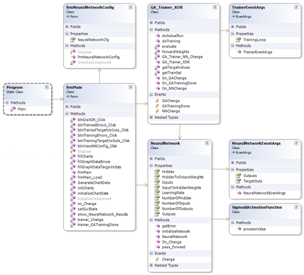
The main classes that people should take the time to look at would be:
GA_Trainer_XOR: Trains a neural network to solve the XOR problem using a Microbial GA.TrainerEventArgs: Training event args, for use with a GUI.NeuralNetwork: A configurable neural network.NeuralNetworkEventArgs: Training event args, for use with a GUI.SigmoidActivationFunction: A static method to provide the sigmoid activation function.
The rest are the GUI I constructed simply to show how it all fits together.
Note: The demo project contains all code, so I won't list it here. Also note that most of these classes are quite similar to those included with the Part 2 article code. I wanted to keep the code similar so people who have already looked at Part 2 would recognize the common pattern.
Code Demos
The demo application attached has three main areas which are described below:
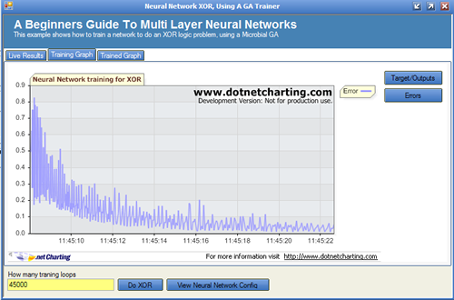
Live Results Tab

It can be seen that this has very nearly solved the XOR problem; it did however take nearly 45000 iterations (epoch) of a training loop. Remembering that we have to also present the entire training set to the network, and also do this twice, once to find a winner and once to find a loser. That is quite a lot of work; I am sure you would all agree. This is why neural networks are not normally trained by GAs; this article is really about how to apply a GA to a problem domain. Because the GA training took 45000 epochs to yield an acceptable result does not mean that GAs are useless. Far from it, GAs have their place, and can be used for many problems, such as:
- Sudoko solver (the popular game)
- Backpack problem (trying to optimize the use of a backpack of limited size, to get as many items in as will fit)
- Favourite pizza toppings problem (try and find out what someone's favourite pizza is)
To name but a few, basically, if you can come up with the genotype and a Fitness function, you should be able to get a GA to work out a solution. GAs have also been used to grow entire syntax trees of grammar, in order to predict which grammar is more optimal. There is more research being done in this area as I write this article; in fact, there is a nice article on this topic (Gene Expression Programming) by Andrew Krillov, right here at the CodeProject, if anyone wants to read further.
Training Results Tab
Viewing the target/outputs together:

Viewing the errors:
Trained Results Tab
Viewing the target/outputs together:

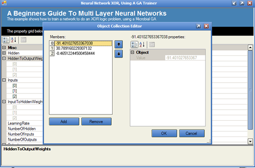
It is also possible to view the neural network's final configuration using the "View Neural Network Config" button.
What Do You Think?
That is it; I would just like to ask, if you liked the article, please vote for it.
Points of Interest
I think AI is fairly interesting, that's why I am taking the time to publish these articles. So I hope someone else finds it interesting, and that it might help further someone's knowledge, as it has my own.
Anyone that wants to look further into AI type stuff, that finds the content of this article a bit basic, should check out Andrew Krillov's articles at Andrew Krillov CP articles as his are more advanced, and very good.
History
- v1.1: 27/12/06: Modified the
GA_Trainer_XORclass to have a random number seed of 5. - v1.0: 11/12/06: Initial article.
Bibliography
- Artificial Intelligence 2nd edition, Elaine Rich / Kevin Knight. McGraw Hill Inc.
- Artificial Intelligence, A Modern Approach, Stuart Russell / Peter Norvig. Prentice Hall.
0 comments:
Post a Comment