from __future__ import absolute_import, division, print_function, unicode_literals
import tensorflow as tf
import matplotlib.pyplot as pltimport matplotlib.ticker as tickerfrom sklearn.model_selection import train_test_split
import unicodedataimport reimport numpy as npimport osimport ioimport time
Download and prepare the dataset
We'll use a language dataset provided by http://www.manythings.org/anki/. This dataset contains language translation pairs in the format:
May I borrow this book? ¿Puedo tomar prestado este libro?
There are a variety of languages available, but we'll use the English-Spanish dataset. For convenience, we've hosted a copy of this dataset on Google Cloud, but you can also download your own copy. After downloading the dataset, here are the steps we'll take to prepare the data:
- Add a start and end token to each sentence.
- Clean the sentences by removing special characters.
- Create a word index and reverse word index (dictionaries mapping from word → id and id → word).
- Pad each sentence to a maximum length.
# Download the file
path_to_zip = tf.keras.utils.get_file(
    'spa-eng.zip', origin='http://storage.googleapis.com/download.tensorflow.org/data/spa-eng.zip',
    extract=True)

path_to_file = os.path.dirname(path_to_zip)+"/spa-eng/spa.txt"
Downloading data from http://storage.googleapis.com/download.tensorflow.org/data/spa-eng.zip
2646016/2638744 [==============================] - 0s 0us/step
# Converts the unicode file to ascii
def unicode_to_ascii(s):
    return ''.join(c for c in unicodedata.normalize('NFD', s)
        if unicodedata.category(c) != 'Mn')

def preprocess_sentence(w):
    w = unicode_to_ascii(w.lower().strip())

    # creating a space between a word and the punctuation following it
    # eg: "he is a boy." => "he is a boy ."
    # Reference:- https://stackoverflow.com/questions/3645931/python-padding-punctuation-with-white-spaces-keeping-punctuation
    w = re.sub(r"([?.!,¿])", r" \1 ", w)
    w = re.sub(r'[" "]+', " ", w)

    # replacing everything with space except (a-z, A-Z, ".", "?", "!", ",")
    w = re.sub(r"[^a-zA-Z?.!,¿]+", " ", w)

    w = w.rstrip().strip()

    # adding a start and an end token to the sentence
    # so that the model know when to start and stop predicting.
    w = '<start> ' + w + ' <end>'
    return w
en_sentence = u"May I borrow this book?"
sp_sentence = u"¿Puedo tomar prestado este libro?"
print(preprocess_sentence(en_sentence))
print(preprocess_sentence(sp_sentence).encode('utf-8'))
<start> may i borrow this book ? <end>
b'<start> \xc2\xbf puedo tomar prestado este libro ? <end>'
# 1. Remove the accents
# 2. Clean the sentences
# 3. Return word pairs in the format: [ENGLISH, SPANISH]
def create_dataset(path, num_examples):
    lines = io.open(path, encoding='UTF-8').read().strip().split('\n')

    word_pairs = [[preprocess_sentence(w) for w in l.split('\t')]  for l in lines[:num_examples]]

    return zip(*word_pairs)
en, sp = create_dataset(path_to_file, None)
print(en[-1])
print(sp[-1])
<start> if you want to sound like a native speaker , you must be willing to practice saying the same sentence over and over in the same way that banjo players practice the same phrase over and over until they can play it correctly and at the desired tempo . <end>
<start> si quieres sonar como un hablante nativo , debes estar dispuesto a practicar diciendo la misma frase una y otra vez de la misma manera en que un musico de banjo practica el mismo fraseo una y otra vez hasta que lo puedan tocar correctamente y en el tiempo esperado . <end>
def max_length(tensor):
    return max(len(t) for t in tensor)
def tokenize(lang):
  lang_tokenizer = tf.keras.preprocessing.text.Tokenizer(
      filters='')
  lang_tokenizer.fit_on_texts(lang)

  tensor = lang_tokenizer.texts_to_sequences(lang)

  tensor = tf.keras.preprocessing.sequence.pad_sequences(tensor,
                                                         padding='post')

  return tensor, lang_tokenizer
def load_dataset(path, num_examples=None):
# creating cleaned input, output pairs
targ_lang, inp_lang = create_dataset(path, num_examples)
input_tensor, inp_lang_tokenizer = tokenize(inp_lang)
target_tensor, targ_lang_tokenizer = tokenize(targ_lang)
return input_tensor, target_tensor, inp_lang_tokenizer, targ_lang_tokenizerLimit the size of the dataset to experiment faster (optional)
Training on the complete dataset of >100,000 sentences will take a long time. To train faster, we can limit the size of the dataset to 30,000 sentences (of course, translation quality degrades with less data):
# Try experimenting with the size of that dataset
num_examples = 30000
input_tensor, target_tensor, inp_lang, targ_lang = load_dataset(path_to_file, num_examples)
# Calculate max_length of the target tensors
max_length_targ, max_length_inp = max_length(target_tensor), max_length(input_tensor)
# Creating training and validation sets using an 80-20 split
input_tensor_train, input_tensor_val, target_tensor_train, target_tensor_val = train_test_split(input_tensor, target_tensor, test_size=0.2)
# Show length
print(len(input_tensor_train), len(target_tensor_train), len(input_tensor_val), len(target_tensor_val))
24000 24000 6000 6000
def convert(lang, tensor):
  for t in tensor:
    if t!=0:
      print ("%d ----> %s" % (t, lang.index_word[t]))
print ("Input Language; index to word mapping")
convert(inp_lang, input_tensor_train[0])
print ()
print ("Target Language; index to word mapping")
convert(targ_lang, target_tensor_train[0])
Input Language; index to word mapping
1 ----> <start>
22 ----> por
50 ----> favor
456 ----> escucha
3 ----> .
2 ----> <end>

Target Language; index to word mapping
1 ----> <start>
56 ----> please
279 ----> listen
3 ----> .
2 ----> <end>
Create a tf.data dataset
BUFFER_SIZE = len(input_tensor_train)
BATCH_SIZE = 64
steps_per_epoch = len(input_tensor_train)//BATCH_SIZE
embedding_dim = 256
units = 1024
vocab_inp_size = len(inp_lang.word_index)+1
vocab_tar_size = len(targ_lang.word_index)+1

dataset = tf.data.Dataset.from_tensor_slices((input_tensor_train, target_tensor_train)).shuffle(BUFFER_SIZE)
dataset = dataset.batch(BATCH_SIZE, drop_remainder=True)
example_input_batch, example_target_batch = next(iter(dataset))
example_input_batch.shape, example_target_batch.shape
(TensorShape([64, 16]), TensorShape([64, 11]))
Write the encoder and decoder model
মনোযোগ সহ একটি এনকোডার-ডিকোডার মডেলটি প্রয়োগ করুন যা আপনি টেনসরফ্লো নিউরাল মেশিন অনুবাদ (seq2seq) টিউটোরিয়ালে পড়তে পারেন । এই উদাহরণটি API এর আরও সাম্প্রতিক সেট ব্যবহার করে। এই নোটবুকটি seq2seq টিউটোরিয়াল থেকে মনোযোগ সমীকরণ প্রয়োগ করে । নিম্নলিখিত চিত্রটি দেখায় যে প্রতিটি ইনপুট শব্দকে মনোযোগ ব্যবস্থা দ্বারা একটি ওজন নির্ধারণ করা হয় যা ডিকোডার দ্বারা বাক্যটির পরবর্তী শব্দটির পূর্বাভাস দেওয়ার জন্য ব্যবহৃত হয়। নীচের চিত্র এবং সূত্রগুলি লুংয়ের কাগজ থেকে মনোযোগ ব্যবস্থার উদাহরণ ।
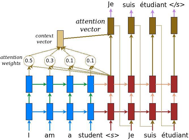
ইনপুটটি একটি এনকোডার মডেলটির মাধ্যমে দেওয়া হয় যা আমাদের আকৃতির এনকোডার আউটপুট দেয় (ব্যাচ_সাইজ, সর্বোচ্চ_ দৈর্ঘ্য, লুকানো_ আকার) এবং এনকোডার লুকানো আকারের আকার (ব্যাচ_সাইজ, লুকানো_সাইজ) ।
এখানে সমীকরণগুলি প্রয়োগ করা হয়েছে:
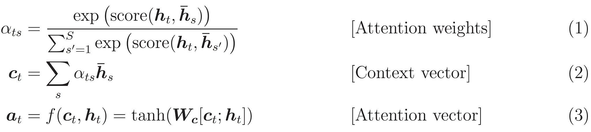
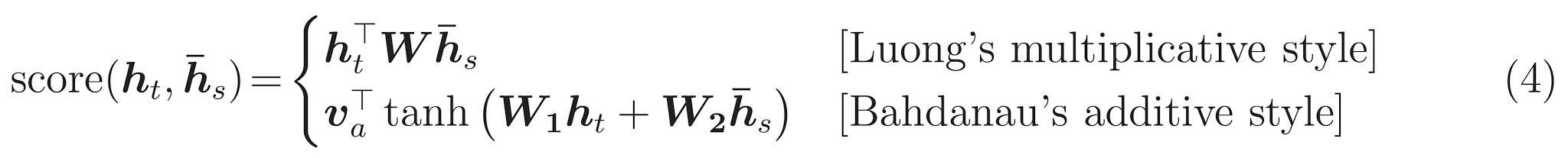
এই টিউটোরিয়ালটি এনকোডারটির জন্য বাহাদানাউ মনোযোগ ব্যবহার করে। সরলিকৃত ফর্মটি লেখার আগে স্বরলিপি সম্পর্কে সিদ্ধান্ত নেওয়া যাক:
- FC = Fully connected (dense) layer
- EO = Encoder output
- H = hidden state
- X = input to the decoder
score = FC(tanh(FC(EO) + FC(H)))
And the pseudo-code:
attention weights = softmax(score, axis = 1)। ডিফল্টরূপে সফটম্যাক্স শেষ অক্ষটিতে প্রয়োগ করা হয় তবে এখানে আমরা এটি 1 ম অক্ষের উপর প্রয়োগ করতে চাই , যেহেতু স্কোরের আকার (ব্যাচ_সাইজ, সর্বোচ্চ_ দৈর্ঘ্য, গোপন_সাইজ) ।Max_lengthআমাদের ইনপুট দৈর্ঘ্য হয়। যেহেতু আমরা প্রতিটি ইনপুটে একটি ওজন নির্ধারণের চেষ্টা করছি, তাই সেই অক্ষের উপর সফটম্যাক্স প্রয়োগ করা উচিত।context vector = sum(attention weights * EO, axis = 1)। অক্ষ হিসাবে 1 হিসাবে বেছে নেওয়ার জন্য উপরের একই কারণ।embedding output= ডিকোডার এক্স এর ইনপুটটি একটি এম্বেডিং স্তরের মধ্য দিয়ে যায়।merged vector = concat(embedding output, context vector)- এই মার্জ করা ভেক্টরটি তখন জিআরইউতে দেওয়া হয়
প্রতিটি পদক্ষেপে সমস্ত ভেক্টরের আকারগুলি কোডের মন্তব্যে নির্দিষ্ট করা হয়েছে:
class Encoder(tf.keras.Model):
  def __init__(self, vocab_size, embedding_dim, enc_units, batch_sz):
    super(Encoder, self).__init__()
    self.batch_sz = batch_sz
    self.enc_units = enc_units
    self.embedding = tf.keras.layers.Embedding(vocab_size, embedding_dim)
    self.gru = tf.keras.layers.GRU(self.enc_units,
                                   return_sequences=True,
                                   return_state=True,
                                   recurrent_initializer='glorot_uniform')

  def call(self, x, hidden):
    x = self.embedding(x)
    output, state = self.gru(x, initial_state = hidden)
    return output, state

  def initialize_hidden_state(self):
    return tf.zeros((self.batch_sz, self.enc_units))
encoder = Encoder(vocab_inp_size, embedding_dim, units, BATCH_SIZE)
# sample input
sample_hidden = encoder.initialize_hidden_state()
sample_output, sample_hidden = encoder(example_input_batch, sample_hidden)
print ('Encoder output shape: (batch size, sequence length, units) {}'.format(sample_output.shape))
print ('Encoder Hidden state shape: (batch size, units) {}'.format(sample_hidden.shape))
Encoder output shape: (batch size, sequence length, units) (64, 16, 1024)
Encoder Hidden state shape: (batch size, units) (64, 1024)
class BahdanauAttention(tf.keras.layers.Layer):
  def __init__(self, units):
    super(BahdanauAttention, self).__init__()
    self.W1 = tf.keras.layers.Dense(units)
    self.W2 = tf.keras.layers.Dense(units)
    self.V = tf.keras.layers.Dense(1)

  def call(self, query, values):
    # hidden shape == (batch_size, hidden size)
    # hidden_with_time_axis shape == (batch_size, 1, hidden size)
    # we are doing this to perform addition to calculate the score
    hidden_with_time_axis = tf.expand_dims(query, 1)

    # score shape == (batch_size, max_length, 1)
    # we get 1 at the last axis because we are applying score to self.V
    # the shape of the tensor before applying self.V is (batch_size, max_length, units)
    score = self.V(tf.nn.tanh(
        self.W1(values) + self.W2(hidden_with_time_axis)))

    # attention_weights shape == (batch_size, max_length, 1)
    attention_weights = tf.nn.softmax(score, axis=1)

    # context_vector shape after sum == (batch_size, hidden_size)
    context_vector = attention_weights * values
    context_vector = tf.reduce_sum(context_vector, axis=1)

    return context_vector, attention_weights
attention_layer = BahdanauAttention(10)
attention_result, attention_weights = attention_layer(sample_hidden, sample_output)
print("Attention result shape: (batch size, units) {}".format(attention_result.shape))
print("Attention weights shape: (batch_size, sequence_length, 1) {}".format(attention_weights.shape))Attention result shape: (batch size, units) (64, 1024)
Attention weights shape: (batch_size, sequence_length, 1) (64, 16, 1)
class Decoder(tf.keras.Model):
  def __init__(self, vocab_size, embedding_dim, dec_units, batch_sz):
    super(Decoder, self).__init__()
    self.batch_sz = batch_sz
    self.dec_units = dec_units
    self.embedding = tf.keras.layers.Embedding(vocab_size, embedding_dim)
    self.gru = tf.keras.layers.GRU(self.dec_units,
                                   return_sequences=True,
                                   return_state=True,
                                   recurrent_initializer='glorot_uniform')
    self.fc = tf.keras.layers.Dense(vocab_size)

    # used for attention
    self.attention = BahdanauAttention(self.dec_units)

  def call(self, x, hidden, enc_output):
    # enc_output shape == (batch_size, max_length, hidden_size)
    context_vector, attention_weights = self.attention(hidden, enc_output)

    # x shape after passing through embedding == (batch_size, 1, embedding_dim)
    x = self.embedding(x)

    # x shape after concatenation == (batch_size, 1, embedding_dim + hidden_size)
    x = tf.concat([tf.expand_dims(context_vector, 1), x], axis=-1)

    # passing the concatenated vector to the GRU
    output, state = self.gru(x)

    # output shape == (batch_size * 1, hidden_size)
    output = tf.reshape(output, (-1, output.shape[2]))

    # output shape == (batch_size, vocab)
    x = self.fc(output)

    return x, state, attention_weights
decoder = Decoder(vocab_tar_size, embedding_dim, units, BATCH_SIZE)
sample_decoder_output, _, _ = decoder(tf.random.uniform((64, 1)),
sample_hidden, sample_output)
print ('Decoder output shape: (batch_size, vocab size) {}'.format(sample_decoder_output.shape))Decoder output shape: (batch_size, vocab size) (64, 4935)
অপ্টিমাইজার এবং ক্ষতি ফাংশন সংজ্ঞায়িত করুন
optimizer = tf.keras.optimizers.Adam()
loss_object = tf.keras.losses.SparseCategoricalCrossentropy(
    from_logits=True, reduction='none')
def loss_function(real, pred):
  mask = tf.math.logical_not(tf.math.equal(real, 0))
  loss_ = loss_object(real, pred)

  mask = tf.cast(mask, dtype=loss_.dtype)
  loss_ *= mask

  return tf.reduce_mean(loss_)
চেকপয়েন্টগুলি (অবজেক্ট-ভিত্তিক সঞ্চয়)
checkpoint_dir = './training_checkpoints'
checkpoint_prefix = os.path.join(checkpoint_dir, "ckpt")
checkpoint = tf.train.Checkpoint(optimizer=optimizer,
                                 encoder=encoder,
                                 decoder=decoder)
প্রশিক্ষণ
- এনকোডার দিয়ে ইনপুটটি পাস করুন যা এনকোডার আউটপুট এবং এনকোডার লুকানো অবস্থায় ফিরে আসে ।
- এনকোডার আউটপুট, এনকোডার লুকানো অবস্থা এবং ডিকোডার ইনপুট (যা শুরু টোকেন ) ডিকোডারে স্থানান্তরিত হয় to
- ডিকোডারটি পূর্বাভাসগুলি এবং ডিকোডার লুকানো অবস্থায় ফিরে আসে ।
- এর পরে ডিকোডার লুকানো অবস্থা আবার মডেলটিতে ফিরে যায় এবং ভবিষ্যদ্বাণীগুলি ক্ষতির গণনা করতে ব্যবহৃত হয়।
- ডিকোডারটিতে পরবর্তী ইনপুট সিদ্ধান্ত নিতে শিক্ষককে বাধ্য করুন Use
- শিক্ষক জোরপূর্বক হ'ল কৌশলটি যেখানে লক্ষ্য শব্দটি ডিকোডারের পরবর্তী ইনপুট হিসাবে পাস করা হয় ।
- চূড়ান্ত পদক্ষেপটি গ্রেডিয়েন্টগুলি গণনা করা এবং এটি অপটিমাইজার এবং ব্যাকপ্রোপগেটে প্রয়োগ করা।
@tf.function
def train_step(inp, targ, enc_hidden):
  loss = 0

  with tf.GradientTape() as tape:
    enc_output, enc_hidden = encoder(inp, enc_hidden)

    dec_hidden = enc_hidden

    dec_input = tf.expand_dims([targ_lang.word_index['<start>']] * BATCH_SIZE, 1)

    # Teacher forcing - feeding the target as the next input
    for t in range(1, targ.shape[1]):
      # passing enc_output to the decoder
      predictions, dec_hidden, _ = decoder(dec_input, dec_hidden, enc_output)

      loss += loss_function(targ[:, t], predictions)

      # using teacher forcing
      dec_input = tf.expand_dims(targ[:, t], 1)

  batch_loss = (loss / int(targ.shape[1]))

  variables = encoder.trainable_variables + decoder.trainable_variables

  gradients = tape.gradient(loss, variables)

  optimizer.apply_gradients(zip(gradients, variables))

  return batch_loss
EPOCHS = 10
for epoch in range(EPOCHS):
start = time.time()
enc_hidden = encoder.initialize_hidden_state()
total_loss = 0
for (batch, (inp, targ)) in enumerate(dataset.take(steps_per_epoch)):
batch_loss = train_step(inp, targ, enc_hidden)
total_loss += batch_loss
if batch % 100 == 0:
print('Epoch {} Batch {} Loss {:.4f}'.format(epoch + 1,
batch,
batch_loss.numpy()))
# saving (checkpoint) the model every 2 epochs
if (epoch + 1) % 2 == 0:
checkpoint.save(file_prefix = checkpoint_prefix)
print('Epoch {} Loss {:.4f}'.format(epoch + 1,
total_loss / steps_per_epoch))
print('Time taken for 1 epoch {} sec\n'.format(time.time() - start))Epoch 1 Batch 0 Loss 4.5782 Epoch 1 Batch 100 Loss 2.3247 Epoch 1 Batch 200 Loss 1.8299 Epoch 1 Batch 300 Loss 1.7017 Epoch 1 Loss 2.0273 Time taken for 1 epoch 32.79620003700256 sec Epoch 2 Batch 0 Loss 1.5939 Epoch 2 Batch 100 Loss 1.4579 Epoch 2 Batch 200 Loss 1.4302 Epoch 2 Batch 300 Loss 1.3060 Epoch 2 Loss 1.3856 Time taken for 1 epoch 17.484558582305908 sec Epoch 3 Batch 0 Loss 0.9645 Epoch 3 Batch 100 Loss 0.9450 Epoch 3 Batch 200 Loss 0.9626 Epoch 3 Batch 300 Loss 1.0414 Epoch 3 Loss 0.9681 Time taken for 1 epoch 17.044427633285522 sec Epoch 4 Batch 0 Loss 0.6285 Epoch 4 Batch 100 Loss 0.7940 Epoch 4 Batch 200 Loss 0.5498 Epoch 4 Batch 300 Loss 0.6397 Epoch 4 Loss 0.6515 Time taken for 1 epoch 17.429885387420654 sec Epoch 5 Batch 0 Loss 0.4643 Epoch 5 Batch 100 Loss 0.4660 Epoch 5 Batch 200 Loss 0.4049 Epoch 5 Batch 300 Loss 0.4017 Epoch 5 Loss 0.4392 Time taken for 1 epoch 17.022470474243164 sec Epoch 6 Batch 0 Loss 0.2925 Epoch 6 Batch 100 Loss 0.2970 Epoch 6 Batch 200 Loss 0.2859 Epoch 6 Batch 300 Loss 0.2650 Epoch 6 Loss 0.3011 Time taken for 1 epoch 17.285199642181396 sec Epoch 7 Batch 0 Loss 0.2012 Epoch 7 Batch 100 Loss 0.1468 Epoch 7 Batch 200 Loss 0.2198 Epoch 7 Batch 300 Loss 0.2109 Epoch 7 Loss 0.2155 Time taken for 1 epoch 16.99945044517517 sec Epoch 8 Batch 0 Loss 0.1343 Epoch 8 Batch 100 Loss 0.1683 Epoch 8 Batch 200 Loss 0.1547 Epoch 8 Batch 300 Loss 0.1345 Epoch 8 Loss 0.1589 Time taken for 1 epoch 17.30172872543335 sec Epoch 9 Batch 0 Loss 0.1193 Epoch 9 Batch 100 Loss 0.1181 Epoch 9 Batch 200 Loss 0.1104 Epoch 9 Batch 300 Loss 0.1278 Epoch 9 Loss 0.1278 Time taken for 1 epoch 17.062464952468872 sec Epoch 10 Batch 0 Loss 0.0915 Epoch 10 Batch 100 Loss 0.0890 Epoch 10 Batch 200 Loss 0.1234 Epoch 10 Batch 300 Loss 0.1449 Epoch 10 Loss 0.1016 Time taken for 1 epoch 17.3432514667511 sec
অনুবাদ করা
- মূল্যায়ন ফাংশনটি প্রশিক্ষণের লুপের সমান, আমরা এখানে শিক্ষক জোর করে ব্যবহার করি না except প্রতিটি সময় পদক্ষেপে ডিকোডারের ইনপুট হ'ল লুকানো অবস্থা এবং এনকোডার আউটপুট সহ পূর্ববর্তী ভবিষ্যদ্বাণী।
- যখন মডেলটি শেষ টোকেনটির পূর্বাভাস দেয় তখন ভবিষ্যদ্বাণী করা বন্ধ করুন ।
- এবং প্রতিবার পদক্ষেপের জন্য মনোযোগের ওজন সংরক্ষণ করুন ।
def evaluate(sentence):
    attention_plot = np.zeros((max_length_targ, max_length_inp))

    sentence = preprocess_sentence(sentence)

    inputs = [inp_lang.word_index[i] for i in sentence.split(' ')]
    inputs = tf.keras.preprocessing.sequence.pad_sequences([inputs],
                                                           maxlen=max_length_inp,
                                                           padding='post')
    inputs = tf.convert_to_tensor(inputs)

    result = ''

    hidden = [tf.zeros((1, units))]
    enc_out, enc_hidden = encoder(inputs, hidden)

    dec_hidden = enc_hidden
    dec_input = tf.expand_dims([targ_lang.word_index['<start>']], 0)

    for t in range(max_length_targ):
        predictions, dec_hidden, attention_weights = decoder(dec_input,
                                                             dec_hidden,
                                                             enc_out)

        # storing the attention weights to plot later on
        attention_weights = tf.reshape(attention_weights, (-1, ))
        attention_plot[t] = attention_weights.numpy()

        predicted_id = tf.argmax(predictions[0]).numpy()

        result += targ_lang.index_word[predicted_id] + ' '

        if targ_lang.index_word[predicted_id] == '<end>':
            return result, sentence, attention_plot

        # the predicted ID is fed back into the model
        dec_input = tf.expand_dims([predicted_id], 0)

    return result, sentence, attention_plot
# function for plotting the attention weights
def plot_attention(attention, sentence, predicted_sentence):
fig = plt.figure(figsize=(10,10))
ax = fig.add_subplot(1, 1, 1)
ax.matshow(attention, cmap='viridis')
fontdict = {'fontsize': 14}
ax.set_xticklabels([''] + sentence, fontdict=fontdict, rotation=90)
ax.set_yticklabels([''] + predicted_sentence, fontdict=fontdict)
ax.xaxis.set_major_locator(ticker.MultipleLocator(1))
ax.yaxis.set_major_locator(ticker.MultipleLocator(1))
plt.show()
def translate(sentence):
    result, sentence, attention_plot = evaluate(sentence)

    print('Input: %s' % (sentence))
    print('Predicted translation: {}'.format(result))

    attention_plot = attention_plot[:len(result.split(' ')), :len(sentence.split(' '))]
    plot_attention(attention_plot, sentence.split(' '), result.split(' '))
সর্বশেষতম চেকপয়েন্ট এবং পরীক্ষা পুনরুদ্ধার করুন
# restoring the latest checkpoint in checkpoint_dir
checkpoint.restore(tf.train.latest_checkpoint(checkpoint_dir))
<tensorflow.python.training.tracking.util.CheckpointLoadStatus at 0x7f687502d9e8>
translate(u'hace mucho frio aqui.')
Input: <start> trata de averiguarlo . <end>
Predicted translation: try to figure it out . <end>

translate(u'esta es mi vida.')
Input: <start> esta es mi vida . <end>
Predicted translation: this is my life . <end>

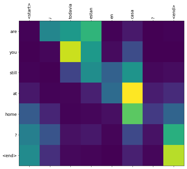
translate(u'¿todavia estan en casa?')
Input: <start> ¿ todavia estan en casa ? <end>
Predicted translation: are we still at home now ? <end>

# wrong translation
translate(u'trata de averiguarlo.')
Input: <start> trata de averiguarlo . <end>
Predicted translation: try to figure it out . <end>

0 comments:
Post a Comment