এটি সম্পাদন করার জন্য, আপনি একটি মনোনিবেশ ভিত্তিক মডেল ব্যবহার করবেন, যা শিরোনাম উত্পন্ন করার সাথে সাথে মডেলটির চিত্রের কোন অংশগুলিতে দৃষ্টি নিবদ্ধ করে তা আমাদের সক্ষম করে।
মডেল আর্কিটেকচারটি শো, উপস্থিতি এবং বলার মতো: ভিজুয়াল মনোযোগ সহ নিউরাল ইমেজ ক্যাপশন জেনারেশন।
এই নোটবুক একটি শেষ থেকে শেষ উদাহরণ। আপনি যখন নোটবুকটি চালান, এটি এমএস-কোকো ডেটাসেট ডাউনলোড করে, ইনসেপশন ভি 3 ব্যবহার করে চিত্রের একটি উপসেট প্রিপ্রোসেসিস এবং ক্যাশে করে, একটি এনকোডার-ডিকোডার মডেল প্রশিক্ষণ দেয় এবং প্রশিক্ষিত মডেলটি ব্যবহার করে নতুন চিত্রগুলিতে ক্যাপশন তৈরি করে।
এই উদাহরণস্বরূপ, আপনি তুলনামূলকভাবে অল্প পরিমাণ ডেটাতে একটি মডেলকে প্রশিক্ষণ দেবেন - প্রায় 20,000 চিত্রের জন্য প্রথম 30,000 ক্যাপশন (কারণ ডেটাশেটে ছবিতে একাধিক ক্যাপশন রয়েছে)।
from __future__ import absolute_import, division, print_function, unicode_literals
import tensorflow as tf
# You'll generate plots of attention in order to see which parts of an image# our model focuses on during captioningimport matplotlib.pyplot as plt
# Scikit-learn includes many helpful utilitiesfrom sklearn.model_selection import train_test_splitfrom sklearn.utils import shuffle
import reimport numpy as npimport osimport timeimport jsonfrom glob import globfrom PIL importImageimport pickle
এমএস-কোকো ডেটাসেটটি ডাউনলোড এবং প্রস্তুত করুন
আপনি আমাদের মডেলটি প্রশিক্ষণ দিতে MS-COCO ডেটাসেট ব্যবহার করবেন। ডেটাসেটে 82,000 এরও বেশি চিত্র রয়েছে, যার প্রতিটিতে কমপক্ষে 5 টি আলাদা ক্যাপশন টিকা রয়েছে ann নীচের কোডটি স্বয়ংক্রিয়ভাবে ডেটাসেটটি ডাউনলোড এবং নিষ্কাশন করে।
Caution: large download ahead. You'll use the training set, which is a 13GB file.
Downloading data from http://images.cocodataset.org/annotations/annotations_trainval2014.zip
252878848/252872794 [==============================] - 8s 0us/step
Downloading data from http://images.cocodataset.org/zips/train2014.zip
12593045504/13510573713 [==========================>...] - ETA: 27s
Optional: limit the size of the training set
এই টিউটোরিয়ালটির প্রশিক্ষণের গতি বাড়ানোর জন্য, আপনি আমাদের মডেলটিকে প্রশিক্ষণ দিতে 30,000 ক্যাপশন এবং তাদের সাথে সম্পর্কিত চিত্রগুলির একটি উপসেট ব্যবহার করবেন। আরও ডেটা ব্যবহার করার সিদ্ধান্ত নেওয়ার ফলে ক্যাপশনের গুণমান উন্নত হবে।
# Read the json filewith open(annotation_file,'r')as f:
annotations = json.load(f)# Store captions and image names in vectors
all_captions =[]
all_img_name_vector =[]for annot in annotations['annotations']:
caption ='<start> '+ annot['caption']+' <end>'
image_id = annot['image_id']
full_coco_image_path = PATH +'COCO_train2014_'+'%012d.jpg'%(image_id)
all_img_name_vector.append(full_coco_image_path)
all_captions.append(caption)# Shuffle captions and image_names together# Set a random state
train_captions, img_name_vector = shuffle(all_captions,
all_img_name_vector,
random_state=1)# Select the first 30000 captions from the shuffled set
num_examples =30000
train_captions = train_captions[:num_examples]
img_name_vector = img_name_vector[:num_examples]
len(train_captions), len(all_captions)
(30000, 414113)
ইনসেপশনভি 3 ব্যবহার করে চিত্রগুলি পূর্ববর্তী করুন
এরপরে, আপনি প্রতিটি চিত্র শ্রেণিবদ্ধ করতে ইনসেপশনভি 3 (যা ইমেজেনেটে পূর্বনির্ধারিত) ব্যবহার করবেন। আপনি শেষ সমাবর্তন স্তর থেকে বৈশিষ্ট্যগুলি নিষ্কাশন করবেন।
প্রথমত, আপনি চিত্রগুলি ইনসেপশনভি 3 এর প্রত্যাশিত বিন্যাসে রূপান্তর করবেন: * চিত্রটি পুনরায় আকার দিয়ে 299px দ্বারা 299px * ছবিটিকে প্রাকৃতিককরণের জন্য প্রাক-প্রসেস_ইনপুট পদ্ধতি ব্যবহার করে চিত্রগুলি প্রসেস করুন যাতে এতে পিক্সেল থাকে -1 থেকে 1 এর মধ্যে, যা মেলে ইনসেপশনভি 3 প্রশিক্ষণ দেওয়ার জন্য ব্যবহৃত চিত্রগুলির ফর্ম্যাট।
ইনসেপশনভি 3 সূচনা করুন এবং প্রাক-প্রশিক্ষিত চিত্রের ওজন লোড করুন
এখন আপনি একটি tf.keras মডেল তৈরি করবেন যেখানে ইনসেপশনভি 3 আর্কিটেকচারের আউটপুট স্তরটি শেষ সমাবর্তন স্তর। এই স্তরটির আউটপুটটির আকার 8x8x2048। আপনি সর্বশেষ সমাবর্তন স্তরটি ব্যবহার করেন কারণ আপনি এই উদাহরণে মনোযোগ ব্যবহার করছেন। প্রশিক্ষণের সময় আপনি এই সূচনাটি সম্পাদন করেন না কারণ এটি কোনও বাধা হয়ে উঠতে পারে।
You forward each image through the network and store the resulting vector in a dictionary (image_name --> feature_vector).
After all the images are passed through the network, you pickle the dictionary and save it to disk.
Downloading data from https://github.com/fchollet/deep-learning-models/releases/download/v0.5/inception_v3_weights_tf_dim_ordering_tf_kernels_notop.h5
87916544/87910968 [==============================] - 3s 0us/step
ইনসেপশনভি 3 থেকে প্রাপ্ত বৈশিষ্ট্যগুলি ক্যাশে করা হচ্ছে
You will pre-process each image with InceptionV3 and cache the output to disk. Caching the output in RAM would be faster but also memory intensive, requiring 8 * 8 * 2048 floats per image. At the time of writing, this exceeds the memory limitations of Colab (currently 12GB of memory).
Performance could be improved with a more sophisticated caching strategy (for example, by sharding the images to reduce random access disk I/O), but that would require more code.
The caching will take about 10 minutes to run in Colab with a GPU. If you'd like to see a progress bar, you can:
# Get unique images
encode_train = sorted(set(img_name_vector))# Feel free to change batch_size according to your system configuration
image_dataset = tf.data.Dataset.from_tensor_slices(encode_train)
image_dataset = image_dataset.map(
load_image, num_parallel_calls=tf.data.experimental.AUTOTUNE).batch(16)for img, path in image_dataset:
batch_features = image_features_extract_model(img)
batch_features = tf.reshape(batch_features,(batch_features.shape[0],-1, batch_features.shape[3]))for bf, p in zip(batch_features, path):
path_of_feature = p.numpy().decode("utf-8")
np.save(path_of_feature, bf.numpy())
Preprocess and tokenize the captions
# Find the maximum length of any caption in our datasetdef calc_max_length(tensor):return max(len(t)for t in tensor)
# Choose the top 5000 words from the vocabulary
top_k =5000
tokenizer = tf.keras.preprocessing.text.Tokenizer(num_words=top_k,
oov_token="<unk>",
filters='!"#$%&()*+.,-/:;=?@[\]^_`{|}~ ')
tokenizer.fit_on_texts(train_captions)
train_seqs = tokenizer.texts_to_sequences(train_captions)
# Create the tokenized vectors
train_seqs = tokenizer.texts_to_sequences(train_captions)
# Pad each vector to the max_length of the captions# If you do not provide a max_length value, pad_sequences calculates it automatically
cap_vector = tf.keras.preprocessing.sequence.pad_sequences(train_seqs, padding='post')
# Calculates the max_length, which is used to store the attention weights
max_length = calc_max_length(train_seqs)
Split the data into training and testing
# Create training and validation sets using an 80-20 split
img_name_train, img_name_val, cap_train, cap_val = train_test_split(img_name_vector,
                                                                    cap_vector,
                                                                    test_size=0.2,
                                                                    random_state=0)
Our images and captions are ready! Next, let's create a tf.data dataset to use for training our model.
# Feel free to change these parameters according to your system's configuration
BATCH_SIZE =64
BUFFER_SIZE =1000
embedding_dim =256
units =512
vocab_size = len(tokenizer.word_index)+1
num_steps = len(img_name_train)// BATCH_SIZE# Shape of the vector extracted from InceptionV3 is (64, 2048)# These two variables represent that vector shape
features_shape =2048
attention_features_shape =64
# Load the numpy filesdef map_func(img_name, cap):
img_tensor = np.load(img_name.decode('utf-8')+'.npy')return img_tensor, cap
dataset = tf.data.Dataset.from_tensor_slices((img_name_train, cap_train))# Use map to load the numpy files in parallel
dataset = dataset.map(lambda item1, item2: tf.numpy_function(
map_func,[item1, item2],[tf.float32, tf.int32]),
num_parallel_calls=tf.data.experimental.AUTOTUNE)# Shuffle and batch
dataset = dataset.shuffle(BUFFER_SIZE).batch(BATCH_SIZE)
dataset = dataset.prefetch(buffer_size=tf.data.experimental.AUTOTUNE)
In this example, you extract the features from the lower convolutional layer of InceptionV3 giving us a vector of shape (8, 8, 2048).
You squash that to a shape of (64, 2048).
This vector is then passed through the CNN Encoder (which consists of a single Fully connected layer).
The RNN (here GRU) attends over the image to predict the next word.
classBahdanauAttention(tf.keras.Model):def __init__(self, units):super(BahdanauAttention,self).__init__()self.W1 = tf.keras.layers.Dense(units)self.W2 = tf.keras.layers.Dense(units)self.V = tf.keras.layers.Dense(1)def call(self, features, hidden):# features(CNN_encoder output) shape == (batch_size, 64, embedding_dim)# hidden shape == (batch_size, hidden_size)# hidden_with_time_axis shape == (batch_size, 1, hidden_size)
hidden_with_time_axis = tf.expand_dims(hidden,1)# score shape == (batch_size, 64, hidden_size)
score = tf.nn.tanh(self.W1(features)+self.W2(hidden_with_time_axis))# attention_weights shape == (batch_size, 64, 1)# you get 1 at the last axis because you are applying score to self.V
attention_weights = tf.nn.softmax(self.V(score), axis=1)# context_vector shape after sum == (batch_size, hidden_size)
context_vector = attention_weights * features
context_vector = tf.reduce_sum(context_vector, axis=1)return context_vector, attention_weights
class CNN_Encoder(tf.keras.Model):# Since you have already extracted the features and dumped it using pickle# This encoder passes those features through a Fully connected layerdef __init__(self, embedding_dim):super(CNN_Encoder,self).__init__()# shape after fc == (batch_size, 64, embedding_dim)self.fc = tf.keras.layers.Dense(embedding_dim)def call(self, x):
x =self.fc(x)
x = tf.nn.relu(x)return x
class RNN_Decoder(tf.keras.Model):def __init__(self, embedding_dim, units, vocab_size):super(RNN_Decoder,self).__init__()self.units = units
self.embedding = tf.keras.layers.Embedding(vocab_size, embedding_dim)self.gru = tf.keras.layers.GRU(self.units,
return_sequences=True,
return_state=True,
recurrent_initializer='glorot_uniform')self.fc1 = tf.keras.layers.Dense(self.units)self.fc2 = tf.keras.layers.Dense(vocab_size)self.attention =BahdanauAttention(self.units)def call(self, x, features, hidden):# defining attention as a separate model
context_vector, attention_weights =self.attention(features, hidden)# x shape after passing through embedding == (batch_size, 1, embedding_dim)
x =self.embedding(x)# x shape after concatenation == (batch_size, 1, embedding_dim + hidden_size)
x = tf.concat([tf.expand_dims(context_vector,1), x], axis=-1)# passing the concatenated vector to the GRU
output, state =self.gru(x)# shape == (batch_size, max_length, hidden_size)
x =self.fc1(output)# x shape == (batch_size * max_length, hidden_size)
x = tf.reshape(x,(-1, x.shape[2]))# output shape == (batch_size * max_length, vocab)
x =self.fc2(x)return x, state, attention_weights
def reset_state(self, batch_size):return tf.zeros((batch_size,self.units))
You extract the features stored in the respective .npy files and then pass those features through the encoder.
The encoder output, hidden state(initialized to 0) and the decoder input (which is the start token) is passed to the decoder.
The decoder returns the predictions and the decoder hidden state.
The decoder hidden state is then passed back into the model and the predictions are used to calculate the loss.
Use teacher forcing to decide the next input to the decoder.
Teacher forcing is the technique where the target word is passed as the next input to the decoder.
The final step is to calculate the gradients and apply it to the optimizer and backpropagate.
# adding this in a separate cell because if you run the training cell# many times, the loss_plot array will be reset
loss_plot =[]
@tf.functiondef train_step(img_tensor, target):
loss =0# initializing the hidden state for each batch# because the captions are not related from image to image
hidden = decoder.reset_state(batch_size=target.shape[0])
dec_input = tf.expand_dims([tokenizer.word_index['<start>']]* BATCH_SIZE,1)with tf.GradientTape()as tape:
features = encoder(img_tensor)for i in range(1, target.shape[1]):# passing the features through the decoder
predictions, hidden, _ = decoder(dec_input, features, hidden)
loss += loss_function(target[:, i], predictions)# using teacher forcing
dec_input = tf.expand_dims(target[:, i],1)
total_loss =(loss /int(target.shape[1]))
trainable_variables = encoder.trainable_variables + decoder.trainable_variables
gradients = tape.gradient(loss, trainable_variables)
optimizer.apply_gradients(zip(gradients, trainable_variables))return loss, total_loss
EPOCHS =20for epoch in range(start_epoch, EPOCHS):
start = time.time()
total_loss =0for(batch,(img_tensor, target))in enumerate(dataset):
batch_loss, t_loss = train_step(img_tensor, target)
total_loss += t_loss
if batch %100==0:print('Epoch {} Batch {} Loss {:.4f}'.format(
epoch +1, batch, batch_loss.numpy()/int(target.shape[1])))# storing the epoch end loss value to plot later
loss_plot.append(total_loss / num_steps)if epoch %5==0:
ckpt_manager.save()print('Epoch {} Loss {:.6f}'.format(epoch +1,
total_loss/num_steps))print('Time taken for 1 epoch {} sec\n'.format(time.time()- start))
Epoch 1 Batch 0 Loss 2.0988
Epoch 1 Batch 100 Loss 1.1463
Epoch 1 Batch 200 Loss 1.0366
Epoch 1 Batch 300 Loss 0.9083
Epoch 1 Loss 1.085102
Time taken for 1 epoch 131.9147825241089 sec

Epoch 2 Batch 0 Loss 0.8748
Epoch 2 Batch 100 Loss 0.7652
Epoch 2 Batch 200 Loss 0.7708
Epoch 2 Batch 300 Loss 0.7578
Epoch 2 Loss 0.812931
Time taken for 1 epoch 49.82423710823059 sec

Epoch 3 Batch 0 Loss 0.8118
Epoch 3 Batch 100 Loss 0.7946
Epoch 3 Batch 200 Loss 0.7396
Epoch 3 Batch 300 Loss 0.6746
Epoch 3 Loss 0.735972
Time taken for 1 epoch 49.87708878517151 sec

Epoch 4 Batch 0 Loss 0.6586
Epoch 4 Batch 100 Loss 0.7100
Epoch 4 Batch 200 Loss 0.6617
Epoch 4 Batch 300 Loss 0.7083
Epoch 4 Loss 0.688551
Time taken for 1 epoch 49.925899028778076 sec

Epoch 5 Batch 0 Loss 0.6543
Epoch 5 Batch 100 Loss 0.6995
Epoch 5 Batch 200 Loss 0.6268
Epoch 5 Batch 300 Loss 0.6577
Epoch 5 Loss 0.650644
Time taken for 1 epoch 49.861159801483154 sec

Epoch 6 Batch 0 Loss 0.6031
Epoch 6 Batch 100 Loss 0.5955
Epoch 6 Batch 200 Loss 0.6627
Epoch 6 Batch 300 Loss 0.5704
Epoch 6 Loss 0.617129
Time taken for 1 epoch 50.251293659210205 sec

Epoch 7 Batch 0 Loss 0.5712
Epoch 7 Batch 100 Loss 0.5685
Epoch 7 Batch 200 Loss 0.5779
Epoch 7 Batch 300 Loss 0.5544
Epoch 7 Loss 0.586807
Time taken for 1 epoch 50.4225971698761 sec

Epoch 8 Batch 0 Loss 0.5429
Epoch 8 Batch 100 Loss 0.5585
Epoch 8 Batch 200 Loss 0.5514
Epoch 8 Batch 300 Loss 0.5229
Epoch 8 Loss 0.555478
Time taken for 1 epoch 50.04306435585022 sec

Epoch 9 Batch 0 Loss 0.5150
Epoch 9 Batch 100 Loss 0.5001
Epoch 9 Batch 200 Loss 0.5294
Epoch 9 Batch 300 Loss 0.5434
Epoch 9 Loss 0.526150
Time taken for 1 epoch 49.535995960235596 sec

Epoch 10 Batch 0 Loss 0.4677
Epoch 10 Batch 100 Loss 0.5044
Epoch 10 Batch 200 Loss 0.4583
Epoch 10 Batch 300 Loss 0.4794
Epoch 10 Loss 0.496457
Time taken for 1 epoch 50.2047655582428 sec

Epoch 11 Batch 0 Loss 0.4150
Epoch 11 Batch 100 Loss 0.4491
Epoch 11 Batch 200 Loss 0.4283
Epoch 11 Batch 300 Loss 0.4874
Epoch 11 Loss 0.465688
Time taken for 1 epoch 50.450185775756836 sec

Epoch 12 Batch 0 Loss 0.4305
Epoch 12 Batch 100 Loss 0.4535
Epoch 12 Batch 200 Loss 0.4198
Epoch 12 Batch 300 Loss 0.4154
Epoch 12 Loss 0.437214
Time taken for 1 epoch 49.61044931411743 sec

Epoch 13 Batch 0 Loss 0.4156
Epoch 13 Batch 100 Loss 0.4067
Epoch 13 Batch 200 Loss 0.4412
Epoch 13 Batch 300 Loss 0.4066
Epoch 13 Loss 0.429518
Time taken for 1 epoch 50.13954949378967 sec

Epoch 14 Batch 0 Loss 0.3823
Epoch 14 Batch 100 Loss 0.4156
Epoch 14 Batch 200 Loss 0.3560
Epoch 14 Batch 300 Loss 0.4084
Epoch 14 Loss 0.387618
Time taken for 1 epoch 49.05424618721008 sec

Epoch 15 Batch 0 Loss 0.3724
Epoch 15 Batch 100 Loss 0.3452
Epoch 15 Batch 200 Loss 0.3371
Epoch 15 Batch 300 Loss 0.3183
Epoch 15 Loss 0.358968
Time taken for 1 epoch 49.87037777900696 sec

Epoch 16 Batch 0 Loss 0.3415
Epoch 16 Batch 100 Loss 0.3094
Epoch 16 Batch 200 Loss 0.3534
Epoch 16 Batch 300 Loss 0.3220
Epoch 16 Loss 0.340680
Time taken for 1 epoch 50.09799098968506 sec

Epoch 17 Batch 0 Loss 0.3501
Epoch 17 Batch 100 Loss 0.3355
Epoch 17 Batch 200 Loss 0.3027
Epoch 17 Batch 300 Loss 0.3440
Epoch 17 Loss 0.318385
Time taken for 1 epoch 49.605764865875244 sec

Epoch 18 Batch 0 Loss 0.3254
Epoch 18 Batch 100 Loss 0.3095
Epoch 18 Batch 200 Loss 0.2968
Epoch 18 Batch 300 Loss 0.2670
Epoch 18 Loss 0.295994
Time taken for 1 epoch 49.70194149017334 sec

Epoch 19 Batch 0 Loss 0.3094
Epoch 19 Batch 100 Loss 0.3093
Epoch 19 Batch 200 Loss 0.2804
Epoch 19 Batch 300 Loss 0.2976
Epoch 19 Loss 0.278130
Time taken for 1 epoch 49.86575794219971 sec

Epoch 20 Batch 0 Loss 0.2911
Epoch 20 Batch 100 Loss 0.2470
Epoch 20 Batch 200 Loss 0.2651
Epoch 20 Batch 300 Loss 0.2656
Epoch 20 Loss 0.258760
Time taken for 1 epoch 50.28017234802246 sec
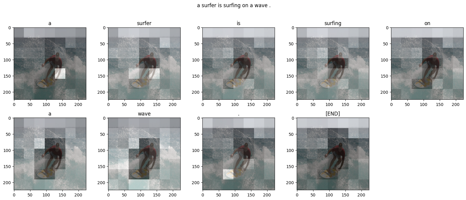
The evaluate function is similar to the training loop, except you don't use teacher forcing here. The input to the decoder at each time step is its previous predictions along with the hidden state and the encoder output.
Stop predicting when the model predicts the end token.
And store the attention weights for every time step.
# captions on the validation set
rid = np.random.randint(0, len(img_name_val))
image = img_name_val[rid]
real_caption =' '.join([tokenizer.index_word[i]for i in cap_val[rid]if i notin[0]])
result, attention_plot = evaluate(image)print('Real Caption:', real_caption)print('Prediction Caption:',' '.join(result))
plot_attention(image, result, attention_plot)# opening the imageImage.open(img_name_val[rid])
Real Caption: <start> a bike parked next to a bucket filled with lots of oranges <end>
Prediction Caption: a man sitting in the banana <end>
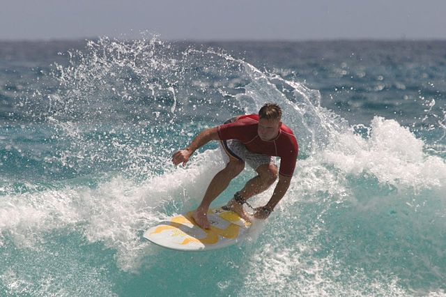
Try it on your own images
For fun, below we've provided a method you can use to caption your own images with the model we've just trained. Keep in mind, it was trained on a relatively small amount of data, and your images may be different from the training data (so be prepared for weird results!)
Downloading data from https://tensorflow.org/images/surf.jpg
65536/64400 [==============================] - 0s 2us/step
Prediction Caption: a man on a surfboard riding a surfboard <end>


0 comments:
Post a Comment