Image segmentation is the process of partitioning an image into multiple different regions (or segments). The goal is to change the representation of the image into an easier and more meaningful image.
It is an important step in image processing, as real world images doesn't always contain only one object that we wanna classify. For instance, for self driving cars, the image would contain the road, cars, pedestrians, etc. So we may need to use segmentation here to separate objects and analyze each object individually (i.e image classification) to check what it is.
In this tutorial, we will see one method of image segmentation, which is K-Means Clustering.
K-Means clustering is unsupervised machine learning algorithm that aims to partition N observations into K clusters in which each observation belongs to the cluster with the nearest mean. A cluster refers to a collection of data points aggregated together because of certain similarities. For image segmentation, clusters here are different image colors.
The following video should make you familiar with K-Means clustering algorithm:
Before we dive into the code, we need to install the required libraries:
pip3 install opencv-python numpy matplotlib
Let's import them:
import cv2
import numpy as np
import matplotlib.pyplot as plt
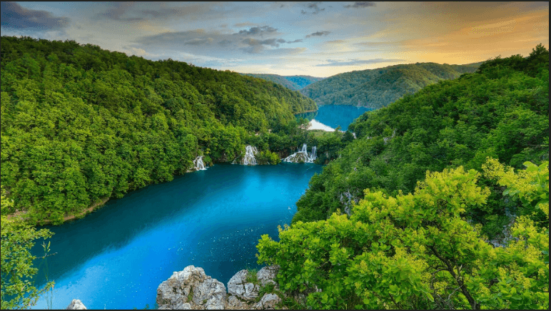
I'm gonna use this image for demonstration purposes, feel free to use any:
Loading the image:
# read the image
image = cv2.imread("image.jpg")
Before we do anything, let's convert the image into RGB format:
# convert to RGB
image = cv2.cvtColor(image, cv2.COLOR_BGR2RGB)
We gonna use cv2.kmeans() function which takes a 2D array as input, and since our original image is 3D (width, height and depth of 3 RGB values), we need to flatten the height and width into a single vector of pixels (3 RGB values):
# reshape the image to a 2D array of pixels and 3 color values (RGB)
pixel_values = image.reshape((-1, 3))
# convert to float
pixel_values = np.float32(pixel_values)
Let's try to print the shape of the resulting pixel values:
print(pixel_values.shape)
Output:
(2073600, 3)
As expected, this is a result of flattening high resolution (1920, 1050) image.
If you watched the video that explains the algorithm, you'll see he says around minute 3 that the algorithm stops when none of the cluster assignments change. Well, we gonna cheat a little bit here, since this is a large number of data points so it'll take a lot of time to process, we are going to stop either when some number of iterations exceeded (say 100) or if the clusters move less than some epsilon value (let's pick 0.2 here), the below code define this stopping criteria in OpenCV:
# define stopping criteria
criteria = (cv2.TERM_CRITERIA_EPS + cv2.TERM_CRITERIA_MAX_ITER, 100, 0.2)
If you look at the image, there are three main colors (green for trees, blue for the sea/lake and white to orange for the sky). As a result, we gonna use three clusters for this image:
# number of clusters (K)
k = 3
_, labels, (centers) = cv2.kmeans(pixel_values, k, None, criteria, 10, cv2.KMEANS_RANDOM_CENTERS)
labels array is the cluster label for each pixel which is either 0, 1 or 2 (since k = 3), centers refers to the center points (each centroid's value).
cv2.KMEANS_RANDOM_CENTERS just indicates OpenCV to randomly assign the values of the clusters initially.
If you look back at the code, we didn't mention that we converted the flattened image pixel values to floats, we did that because cv2.kmeans() expects that, let's convert them back to 8-bit pixel values:
# convert back to 8 bit values
centers = np.uint8(centers)
Now let's construct the segmented image:
# convert all pixels to the color of the centroids
segmented_image = centers[labels.flatten()]
Converting back to the original image shape and showing it:
# reshape back to the original image dimension
segmented_image = segmented_image.reshape(image.shape)
# show the image
plt.imshow(segmented_image)
plt.show()
Here is the resulting image:
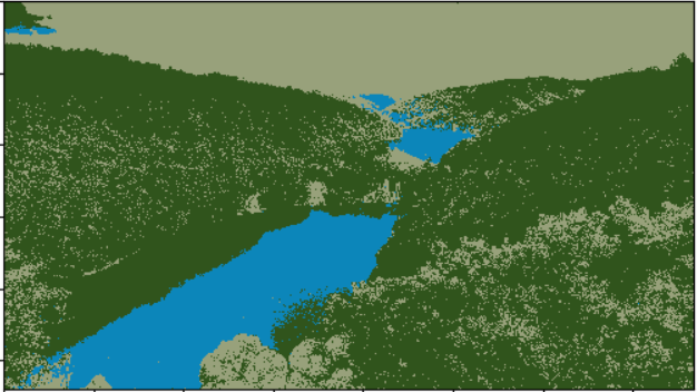
Awesome, we can also disable some clusters in the image. For instance, let's disable the cluster number 2 and show the original image:
# disable only the cluster number 2
masked_image = np.copy(image)
masked_image[labels == 2] = [0, 0, 0]
# show the image
plt.imshow(masked_image)
plt.show()
Here is the resulting image:
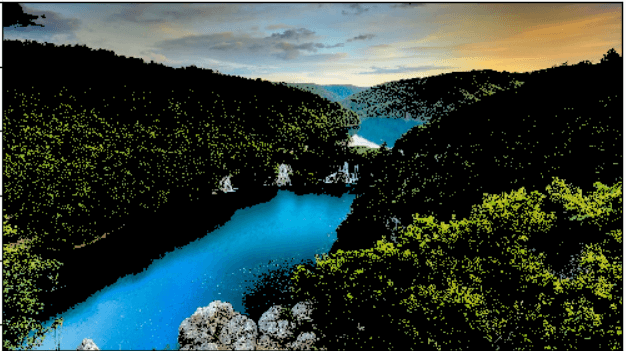
Wow, turns out that cluster 2 is the trees, feel free to:
- Disable other clusters and see which is segmented accurately.
- Tweak the parameters for better results.
- Use better images that clearly contain different objects with different colors.
Note that there are other segmentation techniques such as Hough transform, contour detection and the current state-of-the-art semantic segmentation.
Here are some useful resources:
Code for How to Use K-Means Clustering for Image Segmentation using OpenCV in Python
You can also view the full code on github.
kmeans_segmentation.py
import cv2
import numpy as np
import matplotlib.pyplot as plt

# read the image
image = cv2.imread("image.jpg")

# convert to RGB
image = cv2.cvtColor(image, cv2.COLOR_BGR2RGB)

# reshape the image to a 2D array of pixels and 3 color values (RGB)
pixel_values = image.reshape((-1, 3))
# convert to float
pixel_values = np.float32(pixel_values)

print(pixel_values.shape)
# define stopping criteria
criteria = (cv2.TERM_CRITERIA_EPS + cv2.TERM_CRITERIA_MAX_ITER, 100, 0.2)

# number of clusters (K)
k = 3
compactness, labels, (centers) = cv2.kmeans(pixel_values, k, None, criteria, 10, cv2.KMEANS_RANDOM_CENTERS)

print(labels)
print(centers.shape)

# convert back to 8 bit values
centers = np.uint8(centers)

# convert all pixels to the color of the centroids
segmented_image = centers[labels.flatten()]

# reshape back to the original image dimension
segmented_image = segmented_image.reshape(image.shape)

# show the image
plt.imshow(segmented_image)
plt.show()

# disable only the cluster number 2
masked_image = np.copy(image)
masked_image[labels == 2] = [0, 0, 0]

# show the image
plt.imshow(masked_image)
plt.show()
live_kmeans_segmentation.py (using live cam)
import cv2
import numpy as np

cap = cv2.VideoCapture(0)
k = 5

# define stopping criteria
criteria = (cv2.TERM_CRITERIA_EPS + cv2.TERM_CRITERIA_MAX_ITER, 100, 0.2)

while True:
    # read the image
    _, image = cap.read()

    # reshape the image to a 2D array of pixels and 3 color values (RGB)
    pixel_values = image.reshape((-1, 3))
    # convert to float
    pixel_values = np.float32(pixel_values)

    # number of clusters (K)
    _, labels, (centers) = cv2.kmeans(pixel_values, k, None, criteria, 10, cv2.KMEANS_RANDOM_CENTERS)

    # convert back to 8 bit values
    centers = np.uint8(centers)

    # convert all pixels to the color of the centroids
    segmented_image = centers[labels.flatten()]

    # reshape back to the original image dimension
    segmented_image = segmented_image.reshape(image.shape)

    # reshape labels too
    labels = labels.reshape(image.shape[0], image.shape[1])

    cv2.imshow("segmented_image", segmented_image)
    # visualize each segment

    if cv2.waitKey(1) == ord("q"):
        break

cap.release()
cv2.destroyAllWindows()
0 comments:
Post a Comment