Article Directory
- General framework for machine learning
- SVM background
- SVM introduction
- SVM basic concepts
- SVM algorithm characteristics
- SVM definition and formula establishment
- SVM solution process
- SVM solution case
- SVM application examples
- sklearn simple example
- sklearn divide hyperplane
- Kernel trick
- Motivation to use nuclear methods
- Commonly used kernel functions
- Examples of kernel functions
- Related concepts supplement
- Linear distinguishable and linear indistinguishable
- SVM scales to multiple classification problems
1. General framework for machine learning
Training set => Extracting feature vectors => Combining a certain algorithm (classifier: such as decision tree, KNN) => Get the result
2. SVM background
SVM was first proposed by Vladimir N. Vapnik and Alexey Ya. Chervonenkis in 1963. The current version (soft margin) was proposed by Corinna Cortes and Vapnik in 1993 and published in 1995.
Before the emergence of deep learning (2012), SVM was considered the most successful and best performing algorithm in machine learning in the past ten years.
3. SVM introduction
SVM basic concepts
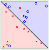
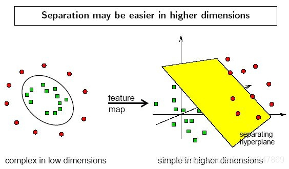
Mapping the feature vectors of the instance (using two dimensions as an example) to some points in space are the solid points and hollow( ফাঁপা) points in the following figure, which belong to two different categories.
Then the purpose of SVM is to draw a line to distinguish the two types of points "best", so that if there are new points in the future, this line can also make a good classification.
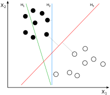
How many lines can be drawn to distinguish the sample points?
: There are countless lines that can be drawn, the difference is that Good effect.
For example, the green line is not good, the blue line is okay, and the red line looks better.
What we hope to findBest effect lineKnown as Dividing the hyperplane
Why is it called "hyperplane"?
: Because the features of the sample are likely to be high-dimensional, the division of the sample space at this time requires a "hyperplane".
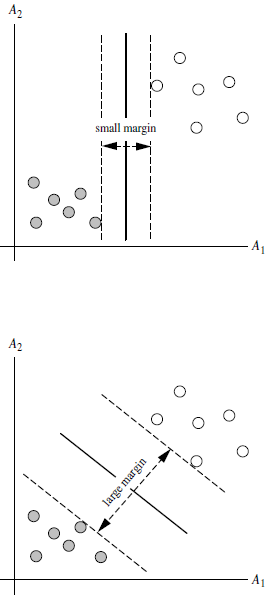
What is the standard for drawing lines? / What makes this line work well?
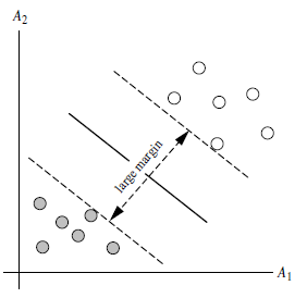
: SVM will look for two classes that can distinguish and enable Maximum margin Hyper plane, ie Dividing the hyperplane.
What is the margin?
: Margin is the sum of the distances of a line from the nearest points on both sides of it.
For example, the band-shaped area formed by the two dashed lines in the figure below is margin, and the dashed line is determined by the two points closest to the central solid line. However, the margin is relatively small at this time. If you use the second method to draw, the margin becomes significantly larger and closer to our goal

Why make the margin as large as possible?
: Because the big margin is less likely to make mistakes
How to choose the Max Margin Hyperplane (MMH)?
: Distance from hyperplane to nearest point on one sideequalThe distance to the nearest point on the other side, the two hyperplanes on both sides are parallel
SVM algorithm characteristics
The algorithm complexity of the trained model is determined byDetermine the number of support vectors, Not by the dimensions of the data. So SVM is less prone to overfitting.
Model trained by SVMTotally dependent on support vectorsEven if all non-support vector points in the training set are removed and the training process is repeated, the result will still get the exact same model.
If the number of support vectors trained by an SVM is relatively small, the model trained by the SVM is easier to generalize.
SVM definition and formula establishment
A hyperplane can be defined as:
wT X+b=0
W: weight vector,
,N is the number of eigenvalues
X: training example
b: bias Assume a 2-dimensional feature vector: X=( x 1 ,x 2 )
Think of b as extra wight, and write it as w0
The hyperplane equation is:
W0+w1x1+w2x2=0
The upper right points of all hyperplanes satisfy:
W0+w1x1+w2x2>0
All points on the lower left of the hyperplane satisfy:
w0+w1x1+w2x2<0
Adjust the weight so that the hyperplane is defined as follows:H
H1:w0+w1x1+w2x2≥1 for yi=+1
H2:w0+w1x1+w2x2≤−1 for yi=−1
Combining the above two formulas, we get:
y i∗(w 0+w 1x 1 +w 2x 2 )≥1, ∀i
All points that lie on the marginal hyperplane are called (support vectors)
Meaning: A support vector is a point that is just pasted on the plane where the margin is located. They are used to define the margin and are the 划分超平面closest points.
Role: The support vector supports the marginal region and is used to establish the division hyperplane.
Note: There may be more than one support vector on one side, and there may be multiple points on one side all attached to the marginal plane.
Divide the distance between the hyperplane and any point on the marginal hyperplane on both sides of it by 1/∣∣w∣∣
(ie: where ∣∣w∣∣ is the norm of a vector (norm))
Therefore, the maximum marginal distance is: 2/|| w ||
The derivation process is to be supplemented.
SVM solution process
How does SVM find the hyperplane with the largest margin (MMH)?
Use some mathematical derivation, formula
y i∗( w0+w 1 x 1+w 2x 2)≥1 , ∀ i can become a restricted quadratic optimization problem
Using Karush-Kuhn-Tucker (KKT) conditions and Lagrangian formula, it can be deduced that MMH can be expressed as the following "decision boundary"

This equation represents the marginally maximized division of the hyperplane.
- L is the number of support vector points, because most points are not support vector points, and only some points on the marginal hyperplane are support vector points. Then we only sum the points that belong to the support vector;
- XiEigenvalues of support vector points;
- yi Is the support vector point Xi The class label, such as +1 or -1;
- X ^ T is the instance to be tested. I want to know which category it belongs to, and bring it into the equation.
- α i And b0Are single numerical parameters, which are obtained by the above-mentioned optimal algorithm, αi Is the Lagrangian multiplier.
Whenever there is a new test sample X , bring it into the equation, see if the value of the equation is positive or negative, and categorize by sign.
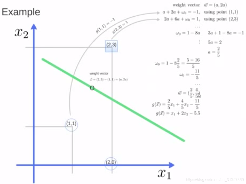
SVM solution case
Take a look at how SVM finds a partitioned hyperplane.
We already know the two support vector points (1,1) and (2,3), set the weight to w = (a, 2a ) , then the coordinates of the two support vector points are brought into the formula respectively w ^ Tx + b = \ ± 1 , you can get:

Then the unknown is a and w_0 , Solve the system of equations:

Bring back the weight vector w has: w=

Then divided hyperplane x_1
 Finally, you can verify with the point (2,0) at the division hyperplane classification results.
SVM application examples
Because the implementation of the SVM algorithm itself is very complicated, we do not study how to implement SVM ourselves, but still use the sklearn library to help us learn the application problem of SVM.
# sklearn import svm module
from sklearn import svm
# Define three points and labels
X = [[2, 0], [1, 1], [2,3]]
y = [0, 0, 1]
# Define classifier, clf means classifier, which is the traditional name of classifier
clf = svm.SVC(kernel = 'linear') # .SVC() is the SVM equation, and the parameter kernel is a linear kernel function
# Training classifier
clf.fit(X, y) # Call the fit function of the classifier to build the model
(that is, calculate the hyperplane division and all relevant attributes are
stored in the classifier cls)
# Print a series of parameters of classifier clf
print (clf)
# Support Vector
print (clf.support_vectors_)
# সমর্থন ভেক্টরের অন্তর্ভুক্ত পয়েন্টের সূচক
print (clf.support_)
# প্রতিটি শ্রেণিতে কয়টি পয়েন্ট সাপোর্ট ভেক্টরের অন্তর্ভুক্ত
print (clf.n_support_)
# একটি নতুন বিষয় পূর্বাভাস
print (clf.predict([[2,0]]))
আউটপুট ফলাফল:
SVC(C=1.0, cache_size=200, class_weight=None, coef0=0.0,
decision_function_shape='ovr', degree=3, gamma='auto_deprecated',
kernel='linear', max_iter=-1, probability=False, random_state=None,
shrinking=True, tol=0.001, verbose=False)
[[1. 1.]
[2. 3.]]
[1 2]
[1 1]
[0]
- এটি দেখা যায় যে SVM - র দ্বারা পাওয়া সহায়তা ভেক্টরগুলি (1,1) এবং (2,3), যা আমাদের উদাহরণের সাথে সামঞ্জস্য করে।
- সমর্থন ভেক্টরের অন্তর্ভুক্ত পয়েন্টগুলির index গুলি 1 এবং 2 হয়
- যেহেতু দুটি সমর্থন ভেক্টর ধনাত্মক এবং নেতিবাচক শ্রেণীর অন্তর্গত পাওয়া গেছে, তাই প্রতিটি শ্রেণীর আউটপুটে সাপোর্ট ভেক্টরের সাথে সম্পর্কিত পয়েন্টগুলির সংখ্যা 1 এবং 1
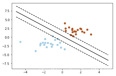
print(__doc__)
# Import related packages
import numpy as np
import pylab as pl # Drawing function
from sklearn import svm
# Create 40 points
np.random.seed(0)
# Leave the random sample points generated by each run of the program unchanged
# Generate training examples and guarantee linear separability
# np._r means connect the matrices in the row direction
# random.randn (a, b) means generate a matrix with a row and b column, and the random numbers obey the standard normal distribution
# array (20,2)-[2,2] is equivalent to subtracting 2 from each number in each row
X = np.r_[np.random.randn(20, 2) - [2, 2], np.random.randn(20, 2) + [2, 2]]
# Two categories each with 20 points, Y is a column vector of 40 rows and 1 column20 টি পয়েন্ট সহ প্রতিটি দুটি বিভাগ, ওয়াই হ'ল 40 টি সারি এবং 1 কলামের কলাম ভেক্টর.
Y = [0] * 20 + [1] * 20
# Create svm model
clf = svm.SVC(kernel='linear')
clf.fit(X, Y)
# Get divided hyperplane
# Divide the original equation of the hyperplane: w0 + w1 + b = 0
# Turn it into a point-slope equation and treat x0 as x, x1 as y, and b as w2
# Dot slope: y =-(w0 / w1)
w = clf.coef_[0] # w is a two-dimensional data, and coef is w = [w0, w1]
a = -w[0] / w[1] # slope
xx = np.linspace(-5, 5) # generate some continuous values from -5 to 5 (random)
# .intercept [0] gets bias, which is the value of b, and b / w [1] is the intercept.
yy = a * xx - (clf.intercept_[0]) / w[1] # Take in the value of x and get the equation of the line.
# Draw and divide two lines parallel to the hyperplane and passing through the support vector (same slope, different intercepts)
b = clf.support_vectors_ [0] # take the first support vector point
yy_down = a * xx + (b [1]-a * b [0])
b = clf.support_vectors _ [-1] # take the last support vector point
yy_up = a * xx + (b [1]-a * b [0])
# View related parameter values
print ("w:", w)
print ("a:", a)
print ("support_vectors_:", clf.support_vectors_)
print ("clf.coef_:", clf.coef_)
# In scikit-learin, coef_ holds the parameter vector that divides the hyperplane in the linear model. The form is (n_classes, n_features). If n_classes> 1, it is a multi-classification problem, and (1, n_features) is a two-classification problem.
# Draw and divide hyperplane, marginal plane and sample points
pl.plot (xx, yy, 'k-')
pl.plot (xx, yy_down, 'k--')
pl.plot (xx, yy_up, 'k--')
# Circle out support vectors
pl.scatter (clf.support_vectors_ [:, 0], clf.support_vectors_ [:, 1],
s = 80, facecolors = 'none')
pl.scatter (X [:, 0], X [:, 1], c = Y, cmap = pl.cm.Paired)
pl.axis ('tight')
pl.show ()
আউটপুট ফলাফল:
Automatically created module for IPython interactive environment
w: [0.90230696 0.64821811]
a: -1.391980476255765
support_vectors_: [[-1.02126202 0.2408932 ]
[-0.46722079 -0.53064123]
[ 0.95144703 0.57998206]]
clf.coef_: [[0.90230696 0.64821811]]
kernel trick
Motivation to use nuclear methods
Formulas that are solved when converted to an optimization problem in a linear SVM are calculated usingInner product(dot product), where ϕ( X)\ phi (X)ϕ ( X ) is a vector point in the training set that is transformed into a high-dimensional non-linear mapping function.Algorithm complexity is very largeTherefore, we use the kernel function instead of calculating the inner product of the non-linear mapping function.
The inner product of the following kernel functions and non-linear mapping functions is equivalent, but the operation of the kernel function K is much less than the inner product.
K(Xi,Xj)=ϕ(Xi)⋅ϕ(Xj)
Commonly used kernel functions
Polynomial kernel of degree h:
K ( Xi,Xj)=( Xi,Xj+1 )h
Gaussian radial basis function kernel:
K(Xi,Xj)=e−∣∣Xi−Xj∣∣2/2σ2
Sigmoid function kernel :
K(Xi,Xj)=tanh(kXi⋅Xj−δ)
How do I choose which kernel to use?
- According to prior knowledge, such as image classification, RBF (Gaussian Radial Basis Function) is usually used, and RBF is not used for text.
- Try different kernels, depending on the accuracy of the results. Try different kernels, depending on the accuracy of the results.
পূর্বের জ্ঞান অনুসারে, যেমন চিত্রের শ্রেণিবদ্ধকরণ, আরবিএফ (গাউসিয়ান রেডিয়াল বেসিস ফাংশন) সাধারণত ব্যবহৃত হয়, এবং আরবিএফ পাঠ্যের জন্য ব্যবহৃত হয় না।
ফলাফলের নির্ভুলতার উপর নির্ভর করে বিভিন্ন কার্নেল ব্যবহার করে দেখুন। ফলাফলের নির্ভুলতার উপর নির্ভর করে বিভিন্ন কার্নেল ব্যবহার করে দেখুন।
Examples of kernel functions
Suppose you define two vectors:
x= (x 1,x2 ,x3),y=(y ,y2 ,y 3 )

Related concepts supplement
Linear distinguishable and linear indistinguishable
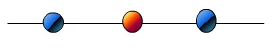
Linear points can be used to classify sample points, otherwise they are linear inseparable.
The following three examples are all linearly indistinguishable, that is, two types of sample points cannot be distinguished by a straight line.
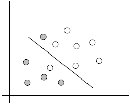
The previous example is linearly distinguishable.
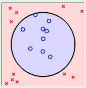
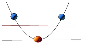
In the case of linear inseparability, the corresponding vector of the data set in space cannot be distinguished by a hyperplane, how to deal with it?
: Two steps to solve:
- Use a non-linear mapping to transform the vector points in the original data set into a higher dimensional space (for example, the following figure maps points in two-dimensional space to three-dimensional space)
- Get a linear space in this high-dimensional processing according to the hyperplane linearly separable case
such desired red and blue dots become linearly separable, then it will map y = x becomes map y= x ^ 2
so that it is linearly separable.
Visual presentation: https://www.youtube.com/watch?v=3liCbRZPrZA

SVM scales to multiple classification problems
The SVM extension can solve multiple classification problems:
for each class, there is a two-class classifier (one-vs-rest) of the current class and other classes that
converts the multi-classification problem into n binary classification problems, where n is the category number.
0 comments:
Post a Comment